TL;DR
If you train Mixture-of-Experts (MoE) transformers, you don't need to re-sweep learning rate, weight decay, or init for every architecture. Tune them once on a small dense FFN proxy, plug the values into a deterministic rule, and they transfer near-optimally to any large MoE configuration — different numbers of activated experts, different total expert counts, different granularities, shared experts, group-balanced routing, width, depth, and batch size.
The recipe is modality-agnostic. The exact same Complete-muE rule (one dense calibration → one transfer table) drives both language modelling and diffusion-based image/video generation — including text-to-image at $256$P / $512$P, $240$P key-frame synthesis, and $240$P $5$s text-to-video. Nothing in the rule is language-specific or vision-specific; it operates on the dense-vs-MoE structural change, which is shared across these architectures.
The whole point is the asymmetry: small dense sweep, large MoE deployment. Our large-scale runs tune at proxy width $d_\star = 128$ and deploy at $d = 1024$ ($8\times$ wider). At that scale the recipe gives $\sim\!4.5\times$ convergence speedup for $240$P $5$s video diffusion, $\sim\!2.5\times$ for $256$P image diffusion, and $\sim\!5.3\text{-}5.5\times$ for LLM training, all versus a dense baseline at the same hyperparameters.
👤 If you're new to MoE, watch the video pairs first, then read why MoE tuning is so painful and continue top-to-bottom.
🛠️ If you train models for a living, jump straight to the recipe and the worked example.
🔬 If you want the math, see how it works (theory) and the "Under the hood" boxes inside it.
See it first: dense vs. MoE samples at identical training cost
Skip the math for a moment. The eight pairs below run on the same text prompts at identical training compute — dense baseline ($\sim$0.62B non-embedding parameters) on the left, MoE 128e8a1s ($\sim$6.3B total, $\sim$0.62B active per token) on the right. The two models are matched in per-token compute — the MoE simply expands total capacity through sparse experts without raising the per-token cost. Both share one hyperparameter setting derived from a single small-dense calibration sweep; there is no per-architecture sweep between them. The MoE side tracks the prompts more faithfully (motion, composition, fidelity) at no extra training budget.
If your reaction after watching is "how would you ever find good MoE hyperparameters without sweeping at this scale?" — that's exactly the question this post answers. The next section names the pain; the one after that shows the numerical proof that the recipe avoids it.
Dense baseline
MoE 128e8a1s
Prompt 1. A Black man in casual attire is filmed in a close head-and-shoulders shot against a clean, neutral seamless backdrop that is entirely free of objects or distractions. The cinematographic composition is centered with shallow depth of field following the rule of thirds, while soft, diffused lighting flatters the subject's face. The camera opens with a handheld dolly-in, physically pushing forward to tighten the frame onto the subject. As the shot settles, the man bursts into a wide, broad smile — his teeth fully visible — his whole face lighting up with unmistakable joy and relaxed warmth.
Dense baseline
MoE 128e8a1s
Prompt 2. At dawn, a vast wind farm stretches across mist-covered fields, towering turbines rotating in the foreground beneath a sky soaked in golden-hour warmth. Long shadows rake across the landscape as saturated, amber light bathes every surface, celebrating the beauty of green energy. The camera begins with a smooth dolly-in that draws the viewer into the scene before transitioning into a controlled wide-angle pan, first centering on the turbines, then slowly widening to reveal the full, sweeping expanse of the farm. The mist, the rotating blades, and the dramatic shadows combine to evoke the quiet power and vastness of renewable energy.
Dense baseline
MoE 128e8a1s
Prompt 3. A vibrant red helicopter soars gracefully above a spectacular panorama of snow-covered mountain peaks glittering beneath a clear blue sky. Bright, hard sunlight floods the scene, creating sharp contrasts between dazzling white snow and deep cerulean sky. The camera holds a steady eye-level distance behind the aircraft, panning smoothly to keep the helicopter continuously centered in frame as it traverses the wide-angle composition. The bold crimson of the helicopter against the pristine alpine wilderness creates a striking visual contrast full of scale and grandeur.
Dense baseline
MoE 128e8a1s
Prompt 4. In the silent depths of outer space, a lone astronaut floats weightlessly before a swirling magnetic field energy wormhole whose luminous glow pulses against a backdrop of stars and distant galaxies. Hard volumetric lighting, intensified by dramatic lens flare, carves the scene into high-contrast relief, while energy particles spiral through the void around the astronaut. The camera holds a static, centered eye-level wide-angle with shallow focus, placing the figure at the heart of the cosmic spectacle. Calm and contemplative, the astronaut observes the cascading energy in a scene that is simultaneously awe-inspiring and serene.
Dense baseline
MoE 128e8a1s
Prompt 5. Several giant woolly mammoths stride purposefully across a serene, snow-blanketed meadow, their long, shaggy fur gently swaying with each lumbering step. Snow-covered trees frame the edges of the wide landscape while dramatic snow-capped mountains rise in the distance beneath a mid-afternoon sky of wispy clouds and warm, diffused sunlight. The camera sits at a low angle, static, its centered shallow-focus composition emphasizing the mammoths' imposing scale against the tranquil, expansive winter world. The soft light and still setting lend the scene an almost mythic, otherworldly calm.
Dense baseline
MoE 128e8a1s
Prompt 6. In close-up, a steaming cup of coffee fills the frame — its frothy surface shimmering under soft, warm light — while two tiny pirate ships, meticulously crafted from sugar and spices, sail and battle across the swirling dark liquid. The camera pans left in a centered, shallow-focus composition, keeping the whimsical miniature vessels sharp against the silky blur of the coffee background. The ships' delicate sails catch the gentle light as they clash in a fierce, fantastical engagement, turning an ordinary cup of coffee into a photorealistic stage for maritime adventure.
Dense baseline
MoE 128e8a1s
Prompt 7. Against a sweeping cinematic aerial view of rolling, snow-covered hills dotted with sparse winter trees, a polar bear — incongruously dressed in a black t-shirt — strums a bass guitar with deliberate, rhythmic intent. Natural daylight falls softly across the scene, casting gentle shadows that reveal the texture of fresh snow and the thick detail of the bear's fur. The camera pans slowly left in a wide-angle, shallow-focus, centered composition, granting full appreciation of the vast, pristine terrain. The bear bobs its head in time with its playing, creating a surreal and delightfully absurd juxtaposition of wilderness and rock-and-roll.
Dense baseline
MoE 128e8a1s
Prompt 8. A cozy living room bathed in warm, inviting light is captured from an elevated overhead perspective in a slow, deliberate pan across the space. The centered, shallow-focus composition draws attention to a large blank picture frame at the room's heart, encircled by an abundance of lush green potted plants that soften the neutral-toned interior. No action disturbs the scene; instead, the slow camera movement becomes the sole motion, guiding the viewer's eye through the tranquil arrangement and allowing the room's peaceful, plant-filled atmosphere to speak entirely for itself.
128e8a1s, at matched training compute and a single set of dense-tuned hyperparameters. Prompts span human portrait, wide landscape, fast-moving subject, abstract cosmic, mythic creatures, photoreal close-up, surreal narrative, and static interior — chosen to stress different aspects of motion, lighting, and composition.Why MoE tuning is so painful
The MoE samples above look like a free lunch from the outside, but the standard path to them is anything but. A modern Mixture-of-Experts transformer block has many knobs you can turn:
- How wide each expert is ($h$)
- How many experts the router activates per token ($a$, "activated experts")
- How many experts exist in total ($N$, "capacity")
- Granularity (more, smaller experts vs. fewer, larger ones)
- Shared experts that always fire
- Group-balanced routing
- ...all on top of the usual width, depth, batch size, and training duration
The catch: each of these choices changes two things at once.
1. The architecture changes
Replacing a dense FFN with an MoE block, or making the experts smaller, alters the parameterized network. Signals propagate differently. Per-step update sizes shift.
2. The data each expert sees changes
An expert only trains on tokens that the router sends to it. With $a$ activated experts out of $N$, each expert sees roughly $a/N$ of the tokens. Change $a$ or $N$ and you've changed each expert's effective batch size and total training duration.
This double-change — shifting update sizes on one side, shifting per-expert workload on the other — is exactly what existing transfer rules cannot handle:
- $\mu\text{P}$1 handles changes to a fixed parameterized model very well — it gives you zero-shot width transfer. Subsequent work extends it to depth, practical training, and diffusion transformers2,3,10. But plain $\mu\text{P}$ has no slot for the per-expert workload.
- SDE-based batch/duration rules4 handle changes in tokens-per-step for a fixed architecture. They don't apply when the architecture itself changes.
- Recent MoE-specific transfer studies5,6 preserve learning-rate ranges under expert-count sweeps but stop short of one compositional rule for the full MoE design space.
So when you go from dense FFN to MoE, or change the MoE capacity, neither tool alone tells you what learning rate to use. Practitioners end up doing what they always did — another full hyperparameter sweep at the new architecture — and that gets expensive fast. Complete-muE is the compositional rule that closes the gap — and the next section is the numerical proof.
Large-scale evidence: the numbers behind the samples
The samples track what the metrics say. At large scale we trained dense and MoE side by side on both LLM and multi-modal diffusion, all at one hyperparameter setting that came out of a single small-dense calibration sweep. We lead with the LM benchmark numbers — they are the most directly interpretable form of "the recipe worked" — then drop into the underlying training curves and convergence speedups that produced them.
Downstream LLM benchmarks: +4.8 to +6.3 points on average, zero retuning
After 100k steps of LM pretraining at the dense-tuned hyperparameters ($\text{LR} = 5\!\times\!10^{-4}$, $\text{WD} = 0.05$, base init std $= 10^{-2}$), both MoE variants substantially improve the dense baseline's average across 13 standard 5-shot benchmarks:
| Model | SVAMP | MMLU | ARC-Easy | ARC-Chall. | COPA | PIQA | HellaSwag |
|---|---|---|---|---|---|---|---|
| Dense | 7.0 | 25.4 | 64.6 | 33.6 | 70.0 | 72.6 | 56.5 |
MoE 128e8a4g1s |
9.7 | 25.9 | 71.2 | 43.6 | 80.0 | 77.7 | 69.3 |
MoE 128e8a1s |
10.0 | 26.2 | 72.9 | 43.4 | 85.0 | 77.8 | 69.4 |
| Model | WinoGrande | LAMBADA | BoolQ | AGIEval-RC | AGIEval-LR | AGIEval-SAT | Average |
| Dense | 59.0 | 50.5 | 62.6 | 20.9 | 27.3 | 26.2 | 44.3 |
MoE 128e8a4g1s |
65.2 | 61.9 | 63.4 | 22.8 | 27.1 | 20.9 | 49.1 |
MoE 128e8a1s |
66.5 | 63.4 | 63.9 | 27.2 | 24.3 | 27.2 | 50.6 |
Average score: 44.3 → 49.1 for the group-balanced variant and 44.3 → 50.6 for the non-grouped variant — a +4.8 to +6.3 point improvement, at the dense-tuned hyperparameters, with no MoE-specific sweep. Same compute, same optimizer state, just a different architecture wired up with Complete-muE's deterministic rule.
Training-loss curves and convergence speedup across modalities
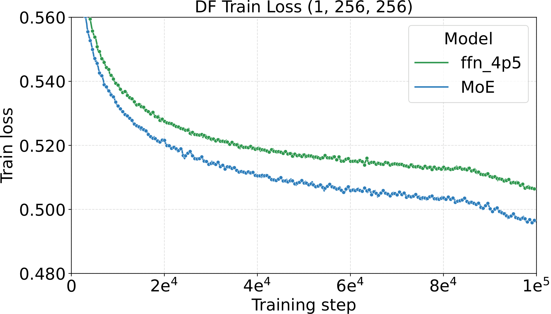
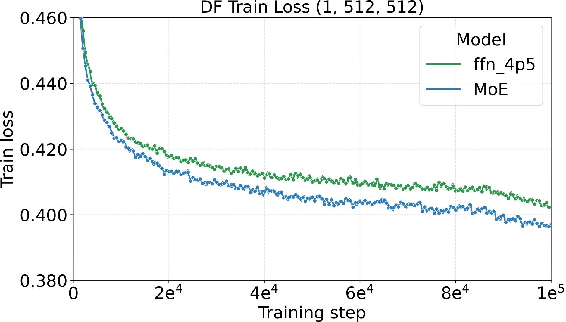
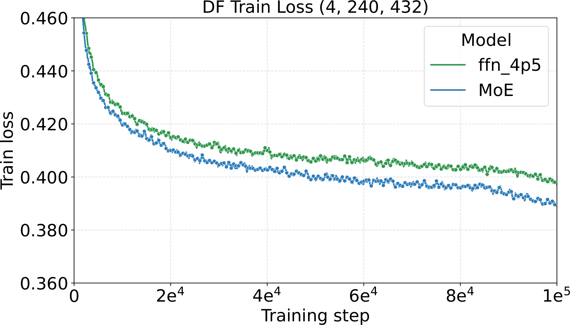
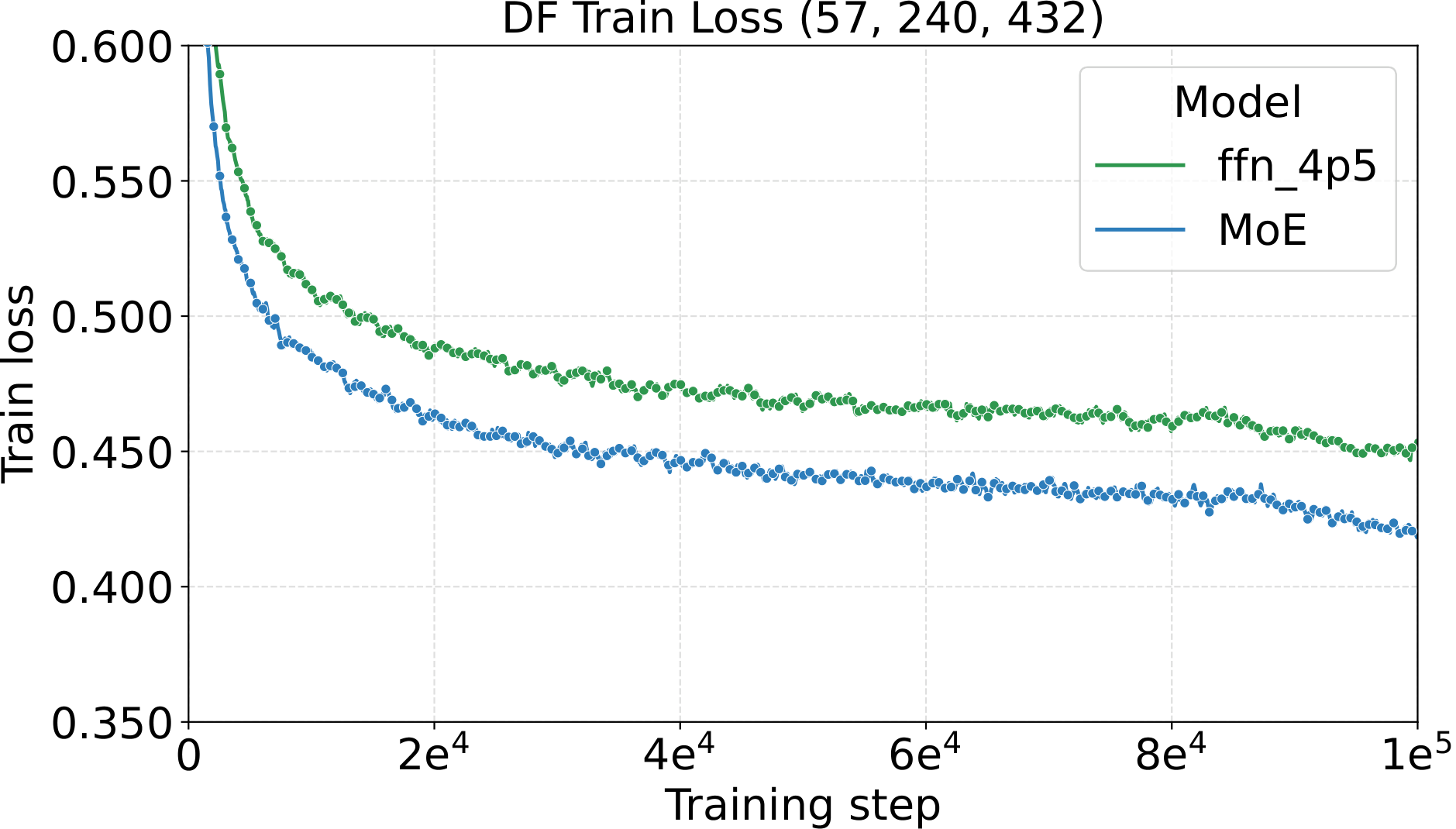
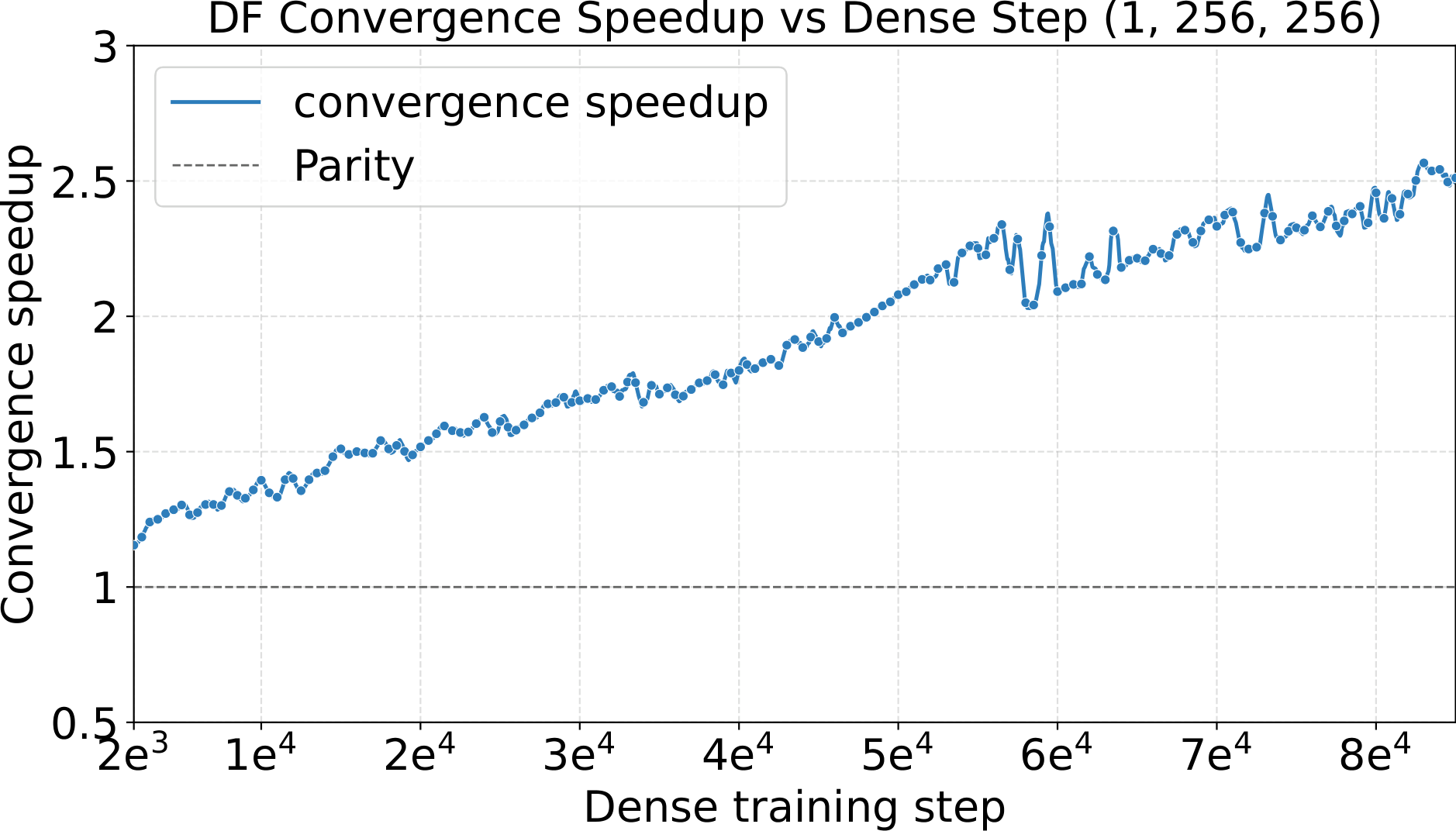
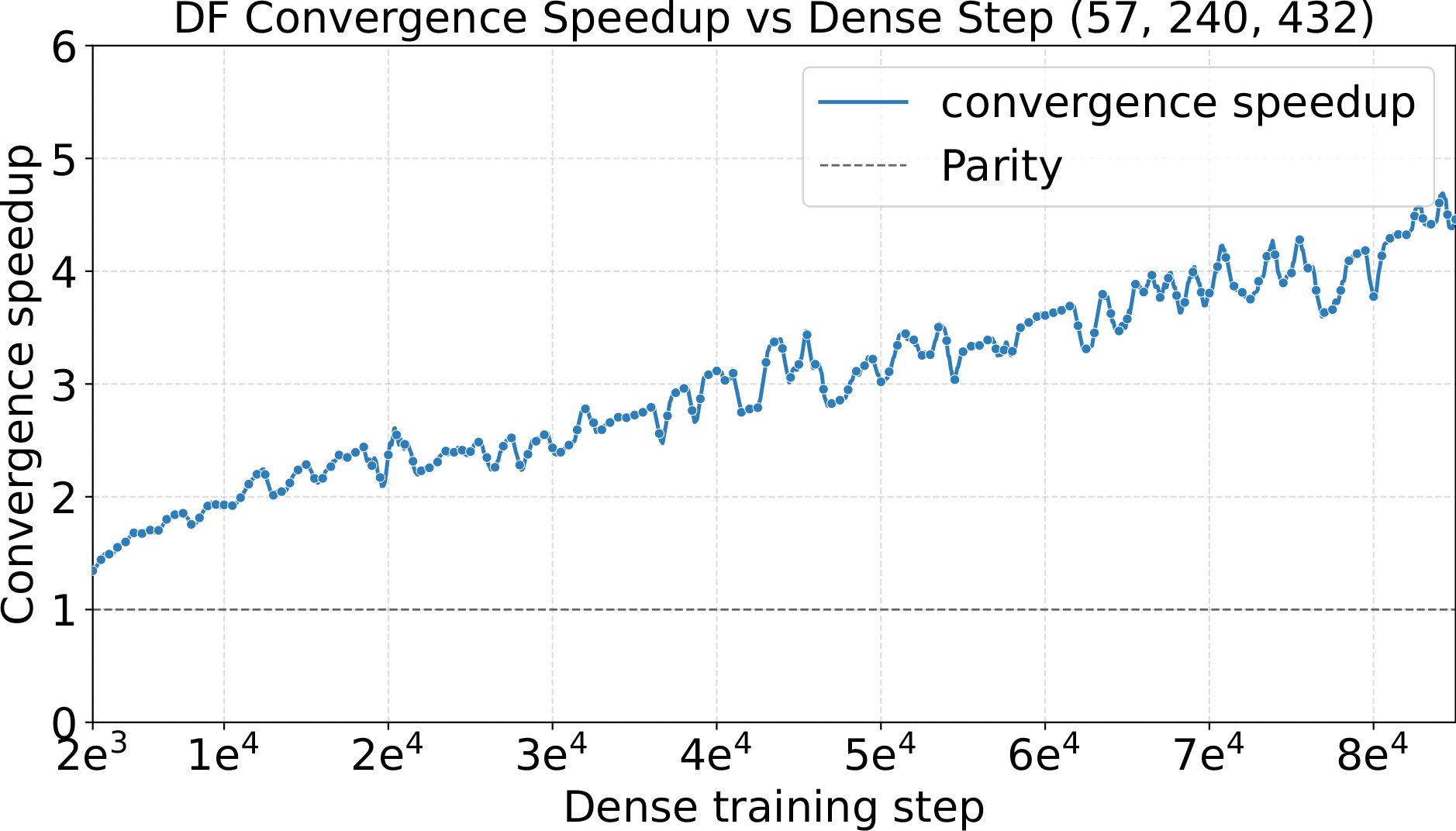
The benchmark gain isn't a one-off: the same pattern appears across every modality we tested. The key asymmetry is tuning on a small dense proxy, deploying at large MoE scale. The calibrated hyperparameters come from short ($25$k–$100$k step) runs at proxy backbone width $d_\star = 128$. The large runs below then use Complete-muE to transfer to backbone width $d = 1024$ ($8\times$ wider, $\sim$6.3B total MoE parameters with $\sim$0.62B active) — a setting that would be prohibitive to sweep directly. The recipe and worked example further down show exactly how the small-proxy values flow into these large runs.
All four multimodal diffusion regimes — $256$P images, $512$P images, $240$P key frames, $240$P $5$s videos — share the diffusion setting from the recipe ($\text{LR} = 2.26\!\times\!10^{-3}$, $\text{WD} = 0.01$, base init std $= 0.02$). The LM run uses the LM setting from the same recipe. The 128e8a1s MoE configuration is the architecture the worked example walks through end-to-end. Each MoE configuration is compared to its dense baseline at those same hyperparameters.
Every setting delivers consistent MoE-over-dense convergence speedup, with no per-setting retuning:
- $\sim\!2.5\times$ on $256$P images
- $\sim\!4.5\times$ on $240$P $5$s videos
- $\sim\!5.3\times$–$5.5\times$ on LLM training (100k iterations)
This is the strongest form of empirical evidence the paper offers: cheap small-dense sweep → expensive large MoE training, across five very different landscapes, all delivering consistent gains.
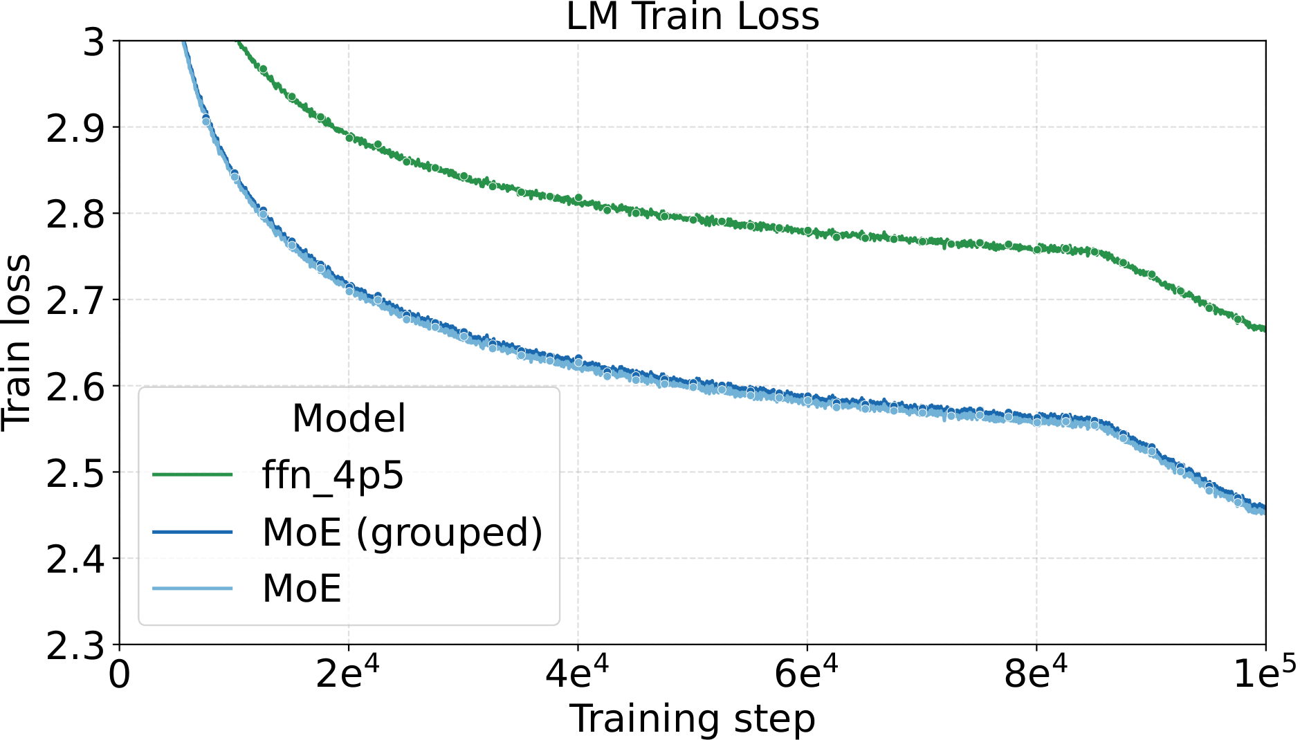
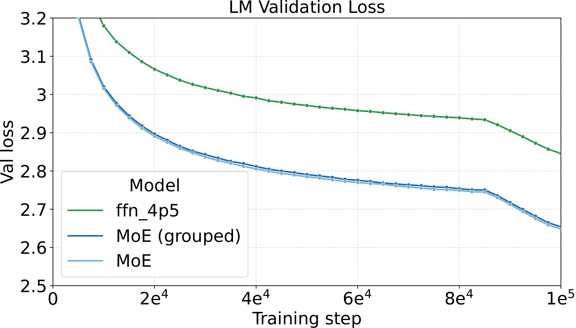
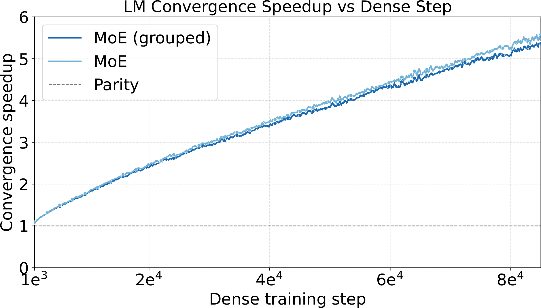
128e8a4g1s and 128e8a1s at one shared hyperparameter setting (LR = $5\times10^{-4}$, WD = $0.05$). Left: smoothed training loss. Middle: validation loss on C4. Right: convergence speedup vs. dense baseline. The MoE variants reach 5.3–5.5× convergence speedup over dense — the training-side counterpart to the +4.8 to +6.3 point benchmark gain in the table above.One last observation about these runs: pretraining with Complete-muE is remarkably stable. Across both the diffusion and LLM settings, training-loss and gradient-norm traces stay smooth for the entire run — essentially free of spikes. A well-calibrated hyperparameter setting does more than improve final loss; it keeps the optimizer in a well-behaved regime where per-step updates are neither too aggressive nor too conservative, avoiding the erratic dynamics that otherwise force costly mid-run interventions or restarts at large MoE scale.
Bonus: large MoEs train at near-dense cost
The results above are about tuning being cheap with Complete-muE. The other half of the practical win is that the training itself — at least along the capacity axis that delivers the largest loss gain (we'll see this in the small-scale evidence further down) — is also cheap. On a single H100 80GB GPU, scaling from $8$ to $256$ total experts (at a fixed $8$ activated) raises step latency only from $87.8$ to $97.0$ ms/step — just $1.08\text{-}1.20\times$ the $81.0$ ms dense SwiGLU baseline. So you can grow MoE parameter count by an order of magnitude while keeping training cost essentially flat.
For context, reaching comparable parameter count by widening a dense model instead would push step latency from $81.0$ to $667.6$ ms ($8\times$ slower) before larger sizes simply run out of memory. The same comparison goes for granularity: fine-grained partitioning ($k = 2 \to 64$) raises latency from $84.1$ to $135.0$ ms/step — not free, but still far cheaper than dense width scaling.
Bottom line: large MoEs trained via capacity scaling are nearly free relative to dense, and Complete-muE makes them tunable for free, too. Both halves of the win compound.
The recipe in three steps
So how do you get the results above? Tune once on a small dense FFN proxy, then compose two short, deterministic tables — one MoE-architectural, one for batch/duration — to transfer those values to any MoE target.
- Tune once on a small dense FFN proxy. Pick a small backbone width (we use $d_\star = 128$), batch size, and a short training duration. Sweep learning rate, weight decay, and initialization on this small dense reference. This is the one and only hyperparameter sweep you do — it stays cheap regardless of how large the target MoE will be.
- Read the layer-level rule from the tuning menu below for your target MoE block. Compute the active width, look up the output multiplier $A$, the route scale $R$, and the down-projection initialization, then apply them.
- Compose the global AdamW factors from the tuning menu's batch/duration section for any width / depth / batch / duration changes. For MoE-specific changes (different $a$, $N$, granularity, shared experts, group-balanced routing), no extra multiplier is needed — the layer-level rule already absorbed those.
The tuning menu below fits on one screen. You do not need to re-sweep for any MoE setting once the dense reference is tuned.
Worked example: small dense → large MoE (128e8a1s)
This is the recipe applied end-to-end: take the small-dense LM and diffusion calibration values, plug them through the two tables, and arrive at the hyperparameters actually used in the large-scale runs. The summary table below shows every knob at both scales; the three steps after it explain where the "Large" column comes from.
Setup — every hyperparameter at a glance
| Small dense proxy | Large MoE (target) | |
|---|---|---|
| Architecture | dense FFN | MoE 128e8a1s (128 routed experts, 8 activated, 1 shared) |
| Backbone width $d$ | $128$ | $1024$ ($\rho_d = 8$) |
| FFN-expansion equivalence | $1\times$ | $4.5\times$ ($H_\mathrm{act}/d = 9$) |
| Training iterations $T$ | $25{,}000$ | $100{,}000$ ($\rho_T = 4$) |
| Batch size | unchanged across scales ($\rho_B = 1$) | |
| Global AdamW hyperparameters (the single LR/WD/init you set in the optimizer) | ||
| LM — base LR | $10^{-3}$ | $5\!\times\!10^{-4}$ |
| LM — weight decay | $0.10$ | $0.05$ |
| LM — init std | $0.01$ | $0.01$ |
| Diffusion — base LR | $4.52\!\times\!10^{-3}$ | $2.26\!\times\!10^{-3}$ |
| Diffusion — weight decay | $0.02$ | $0.01$ |
| Diffusion — init std | $0.02$ | $0.02$ |
| MoE layer-level overrides (applied at the large MoE only) | ||
| Active width $H_\mathrm{act}$ | $d$ (dense) | $9d$ (shared $+$ 8 routed) |
| Output multiplier $A = d/H_\mathrm{act}$ | $1$ | $1/9$ (on FFN/MoE down-projection) |
| Route scale $R$ | $1$ | $8$ on routed sum, $1$ on shared branch |
| Down-proj init-std factor $\sqrt{H_\mathrm{act}/d}$ | $\times 1$ | $\times 3$ (applied on top of dense-baseline init std) |
| μP per-layer scaling (every 2D linear projection inside the transformer block at the large MoE) | ||
| Per-layer LR factor ($\rho_d^{-1}$) | $\times 1$ | $\times 1/8$ |
| Per-layer init-std factor ($\rho_d^{-1/2}$) | $\times 1$ | $\times 1/\sqrt{8}$ |
| Final output-projection multiplier ($1/\rho_d$) | $\times 1$ | $\times 1/8$ (LM head / diffusion output projection) |
Step 1 — global batch/duration scaling (Table 2)
The batch is unchanged; only the duration grows ($T_\star = 25\text{k} \to T = 100\text{k}$). This is the "fixed batch, change duration" row of the tuning menu, with $\rho_B = 1$ and $\rho_D = \rho_B \cdot \rho_T = 4$, so
$$\eta,\lambda \;\;\times\;\; \sqrt{\rho_B/\rho_D} \;=\; \sqrt{1/4} \;=\; 1/2.$$
That halves the base LR and WD between the two columns of the table above — LM: $10^{-3} \to 5\!\times\!10^{-4}$, $0.10 \to 0.05$; diffusion: $4.52\!\times\!10^{-3} \to 2.26\!\times\!10^{-3}$, $0.02 \to 0.01$. Init std is untouched by Step 1 (batch and duration don't enter the initialization rule).
Step 2 — MoE layer-level rule (Table 1)
The 128e8a1s block has 8 routed-active experts plus 1 shared expert, giving an FFN expansion equivalence of $4.5\times$ and an active width $H_\mathrm{act} = 9d$ when shared and routed contributions are combined. The Table 1 lookup for hybrid blocks then gives:
- Output multiplier $A = d/H_\mathrm{act} = 1/9$, applied to the MoE down-projection output.
- Route scale $R = 8$ on the normalized routed sum; the shared branch keeps $R = 1$.
- Down-projection init-std factor $\sqrt{H_\mathrm{act}/d} = \sqrt{9} = 3$, multiplied onto the dense-baseline init std for that one parameter.
No MoE-specific multiplier touches the LR or WD — those changes are fully absorbed by $A$, $R$, and the init-std factor.
Step 3 — standard $\mu\text{P}$ per-layer scaling ($d$: $128 \to 1024$)
Standard $\mu\text{P}$ scales every 2D linear projection inside the transformer block — the FFN/MoE up, gate, and down projections, the router readout, the attention $Q$, $K$, $V$, and $O$ projections, plus anything else that is a learned $d_\text{in} \!\times\! d_\text{out}$ matrix. All of them inherit the same two width factors:
$$\eta_{\text{per-layer}} \;\propto\; \rho_d^{-1} = 1/8, \qquad \sigma_{\text{per-layer}} \;\propto\; \rho_d^{-1/2} = 1/\sqrt{8}.$$
In words: every such linear layer at $d = 1024$ uses $1/8$ the LR and $1/\sqrt{8}$ the init std of the same layer at $d = 128$, before any MoE-specific factors are applied on top.
$\mu\text{P}$ also specifies a separate output multiplier for the final embedding-to-logits (or embedding-to-output) projection — the LM head for language modelling, the noise/velocity prediction head for diffusion. That multiplier is $1/\rho_d$ (the inverse width-expansion ratio). With $\rho_d = 8$ here, the final output projection gets an extra $\times 1/8$ scaling factor, independently of the per-layer LR/init rules above.
Effective per-parameter values at the large MoE
Composing Step 2 (MoE layer rule) with Step 3 ($\mu\text{P}$ width factor) gives the actual per-parameter LR and init std for each parameter group:
| Parameter group | LR factor | Init-std factor | LM init std | DF init std |
|---|---|---|---|---|
| FFN/MoE down-projection | $\times 1/8$ | $\times 3/\sqrt{8} \approx 1.06$ | $\approx 0.0106$ | $\approx 0.0212$ |
| FFN/MoE up & gate projections | $\times 1/8$ | $\times 1/\sqrt{8} \approx 0.354$ | $\approx 0.0035$ | $\approx 0.0071$ |
| Router readout | $\times 1/8$ | $\times 1/\sqrt{8}$ | $\approx 0.0035$ | $\approx 0.0071$ |
| Attention QKVO & other linear layers | $\times 1/8$ | $\times 1/\sqrt{8}$ | $\approx 0.0035$ | $\approx 0.0071$ |
| Final output projection (LM head / DF head) | $\times 1/8$ | $\times 1/\sqrt{8}$ and output multiplier $\times 1/\rho_d = \times 1/8$ | $\approx 0.0035$ | $\approx 0.0071$ |
The final output projection gets both the per-layer $\mu\text{P}$ scaling (Step 3, same as every other 2D linear) and the additional output multiplier $\times 1/\rho_d$ on its output activations. On top of that, the MoE-specific multipliers from Step 2 apply only to the routed-output branch inside the MoE block: output multiplier $A = 1/9$ on the down-projection output, and route scale $R = 8$ on the normalized routed sum (the shared expert keeps $R = 1$).
There is no per-architecture sweep between the small calibration and the large run. Every number in the "Large" column of the setup table is mechanical — it follows from the small-proxy values by applying the two tables in sequence.
Small-scale evidence
The recipe works because of three layered facts: the dense calibration sweep gives broad, well-separated optima (so reuse is forgiving); fixing those values and scaling only the MoE architecture gives consistent loss reductions (the cleanest possible "tune-once" test); and sweeping any AdamW hyperparameter at fixed MoE architecture keeps the optimum in the same window. We show each one in order.
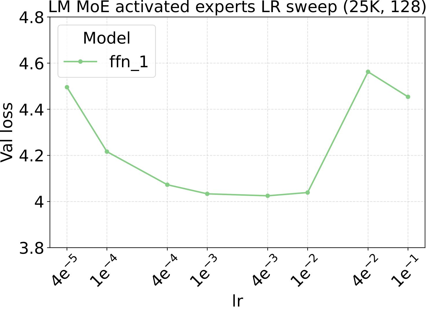
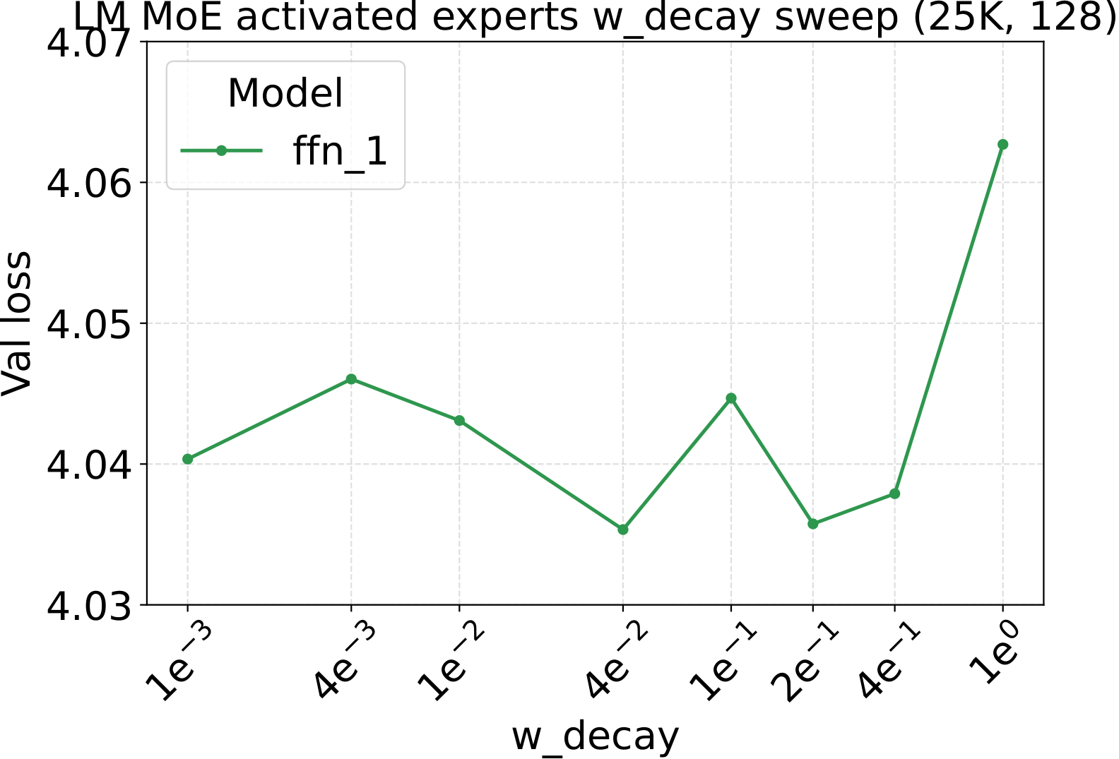
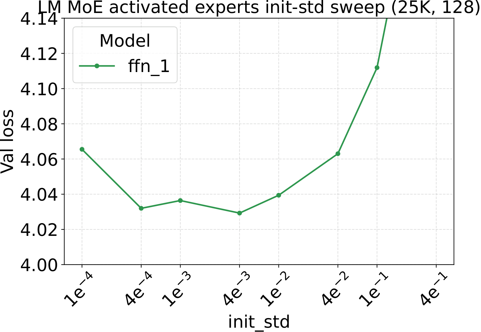
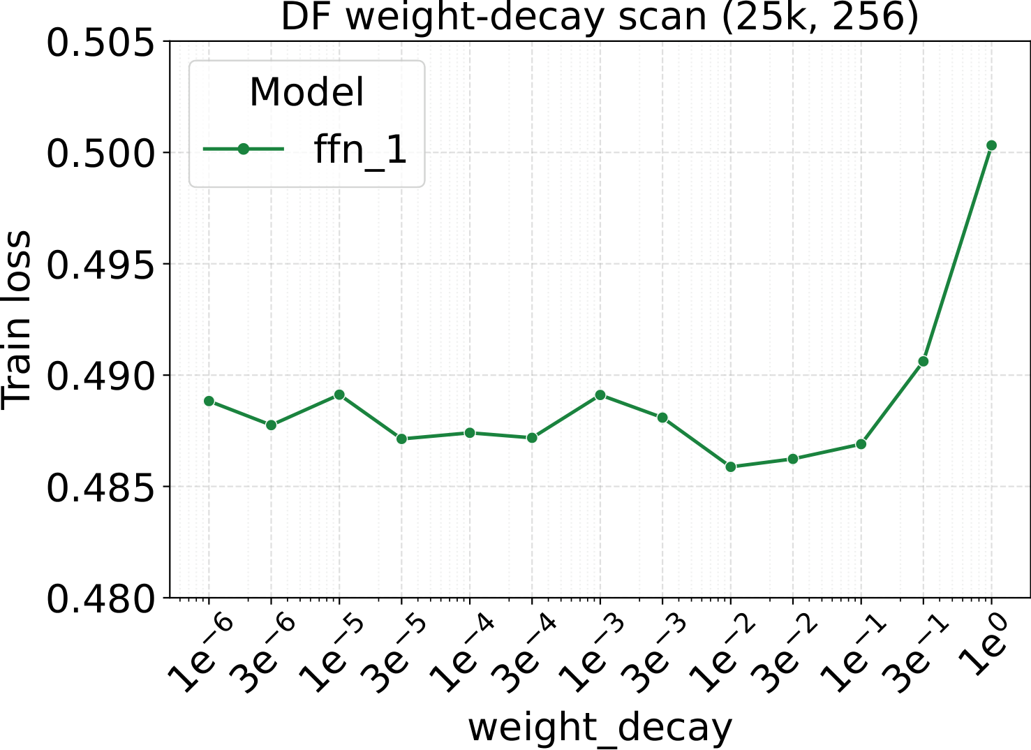
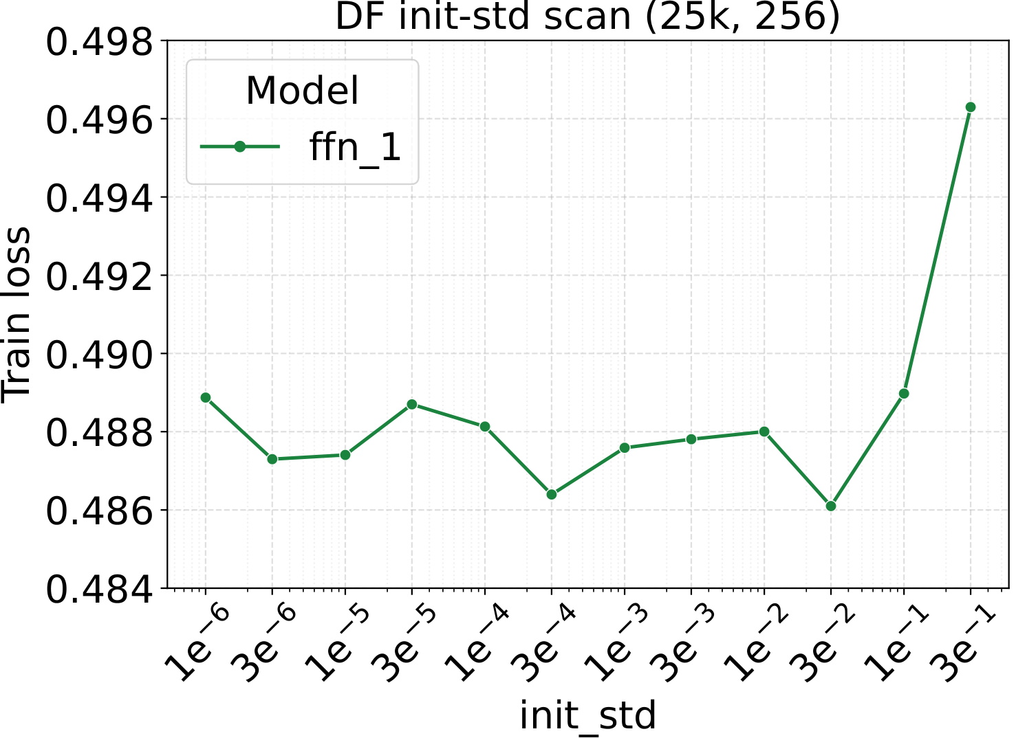
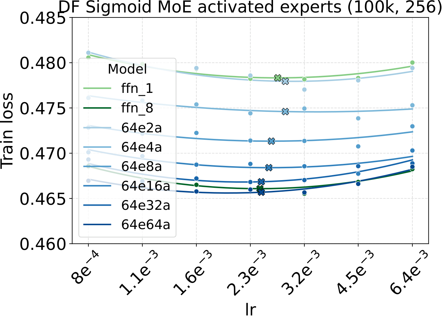
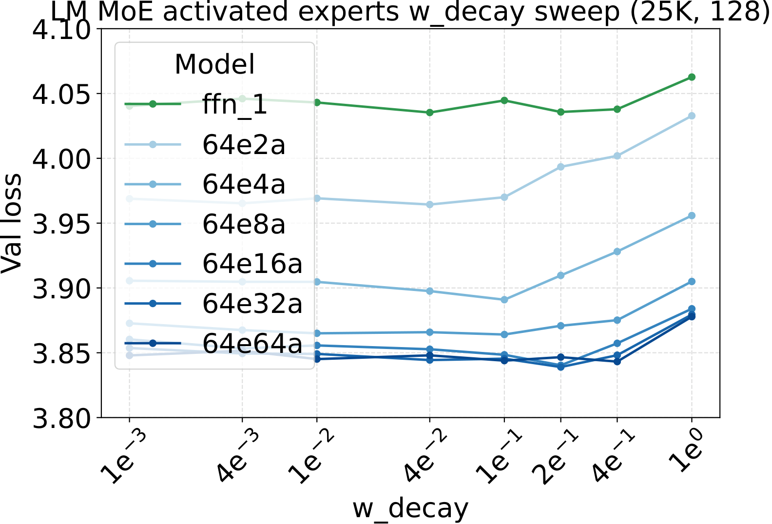
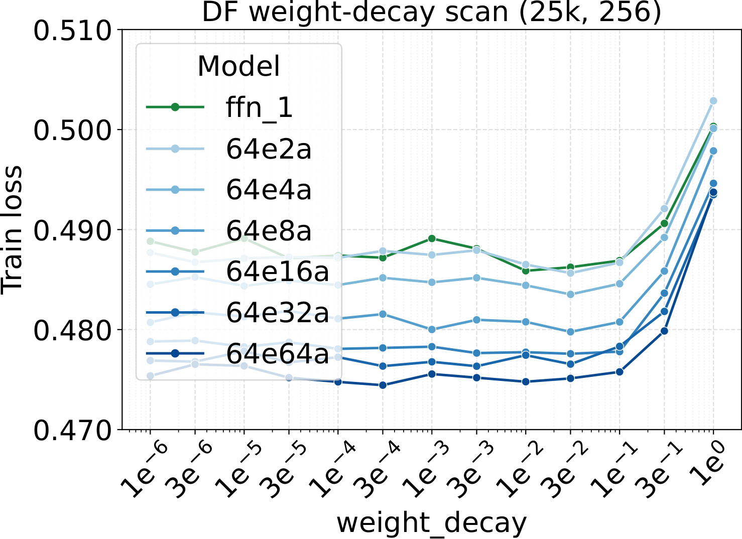
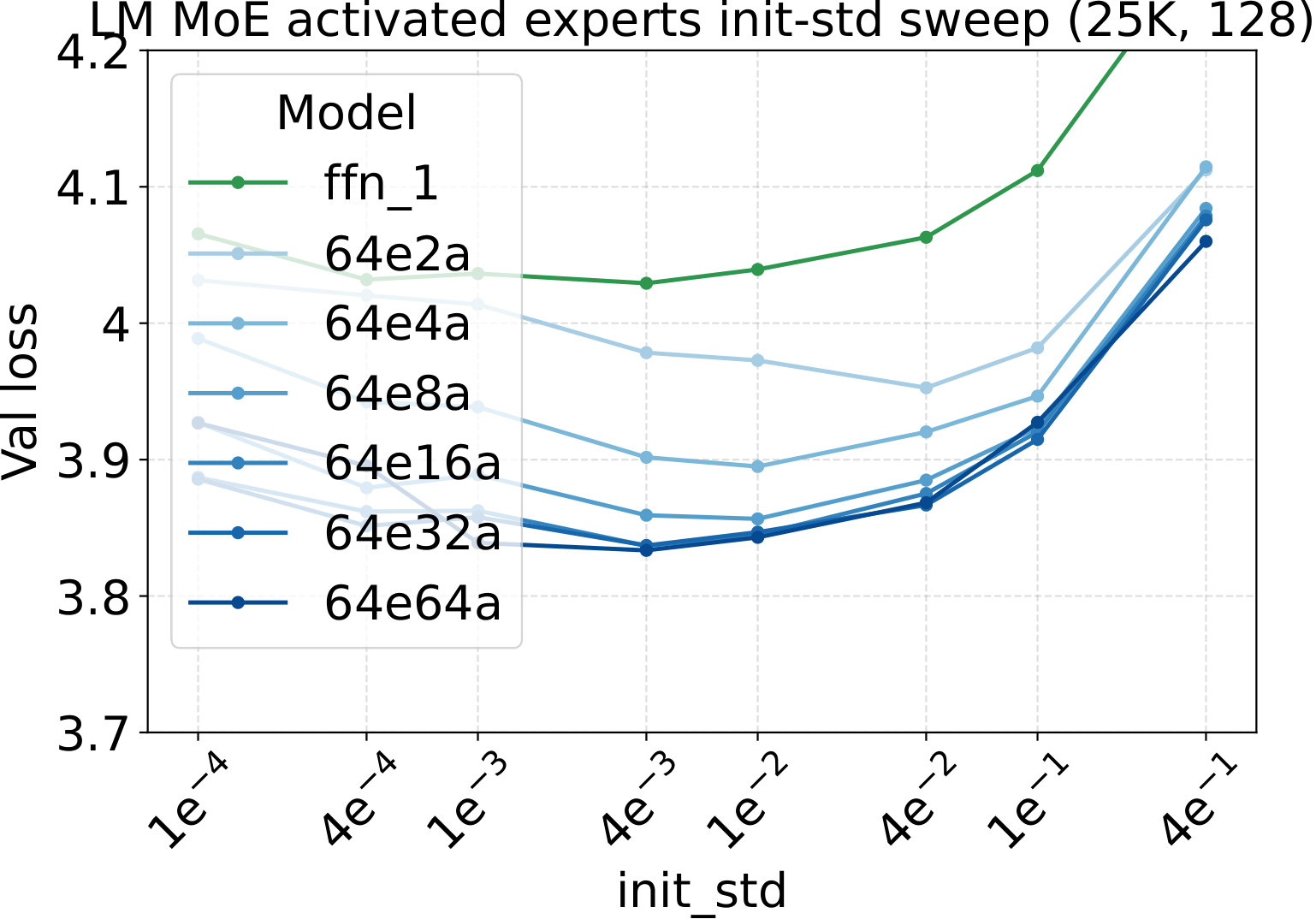
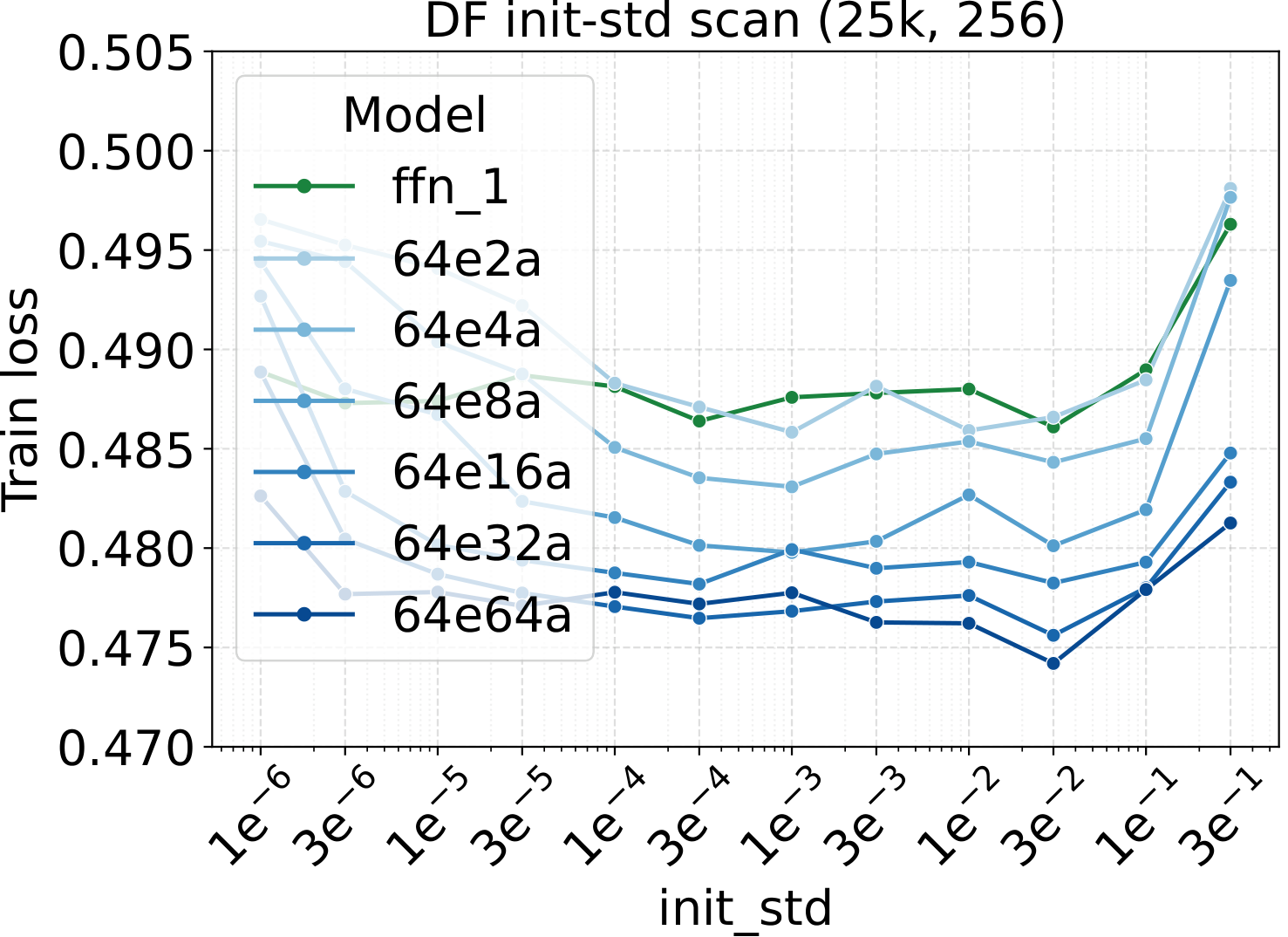
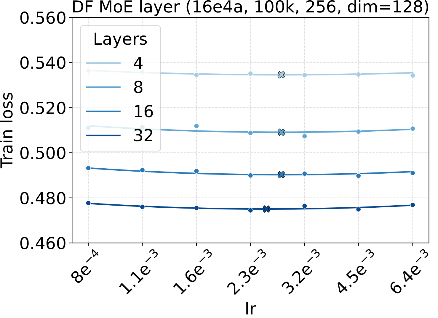
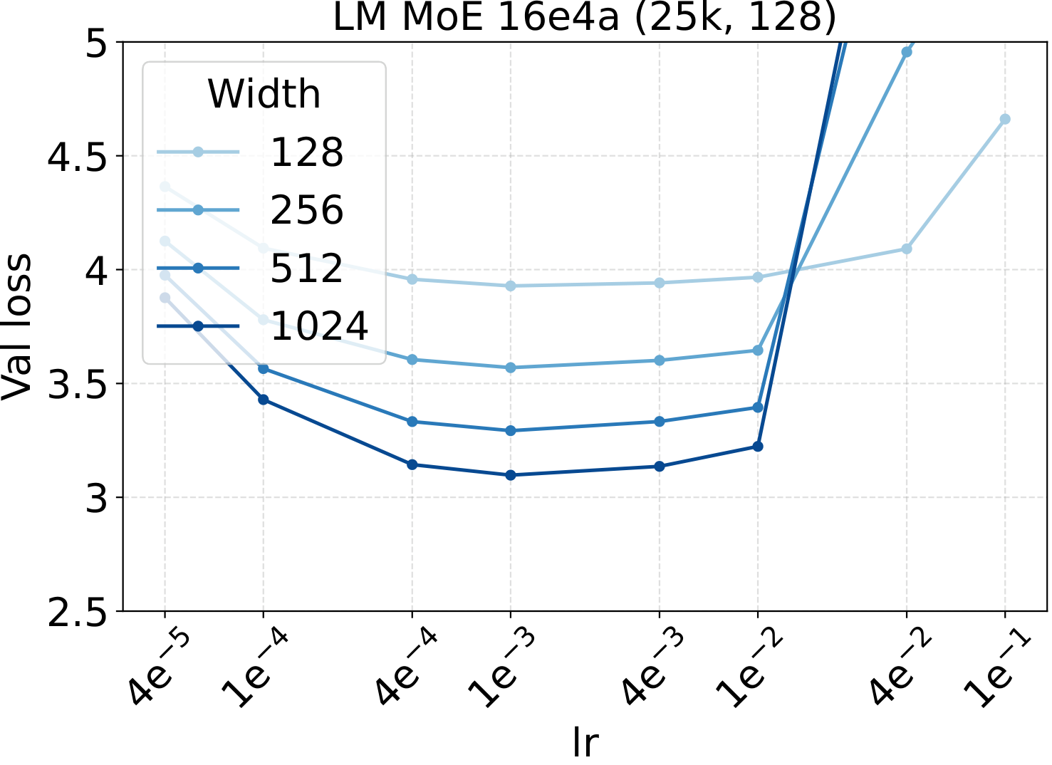
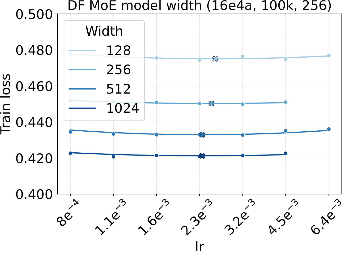
The small-dense calibration sweep
Step 1 of the recipe is a single sweep on a small dense FFN proxy. For both modalities we scan three hyperparameters — learning rate, weight decay, and initialization std — at proxy backbone width $d_\star = 128$. The optima are broad and well-separated, which is what makes them easy to reuse downstream:
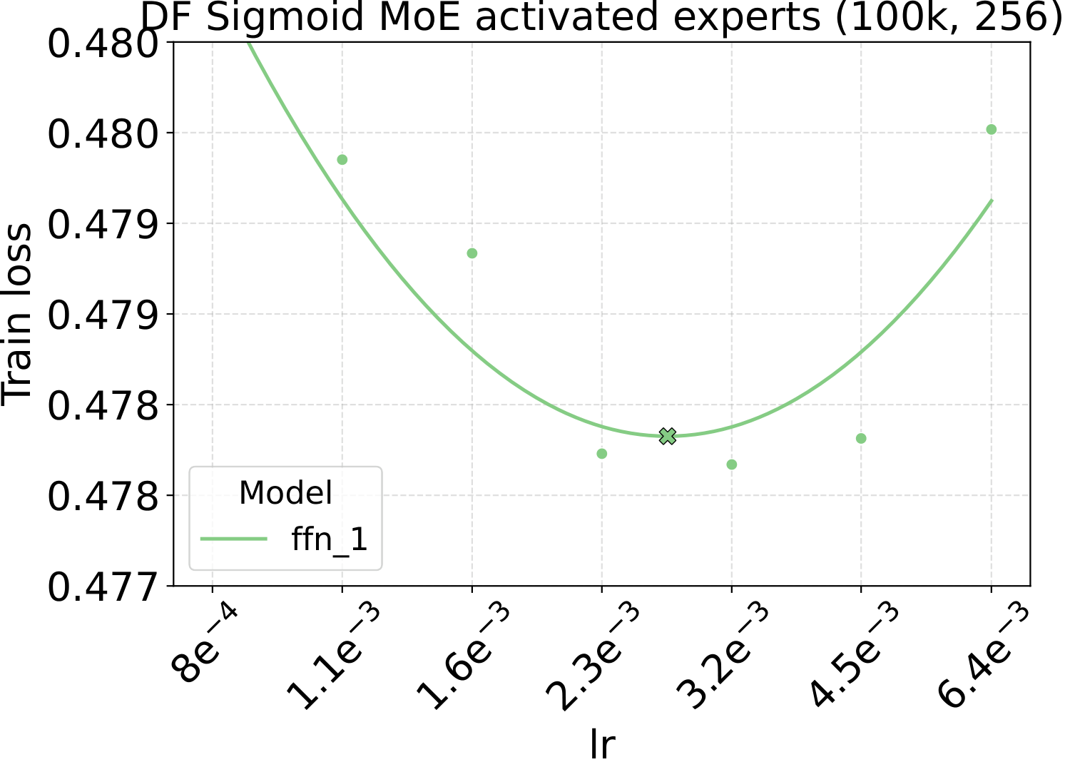
Fixed-LR scaling: the cleanest tune-once test
The most direct check of the recipe is to fix all AdamW hyperparameters at the small-dense calibration values (LM: $\text{LR}=10^{-3}$, $\text{WD}=0.10$, init std $=10^{-2}$; Diffusion: $\text{LR}=4.52\!\times\!10^{-3}$, $\text{WD}=0.02$, init std $=2\!\times\!10^{-2}$) and then scale only the MoE architecture along four axes. If the recipe really is tune-once-and-transfer, loss should drop monotonically and consistently as the architecture grows — no per-setting re-tuning. That is what we see:
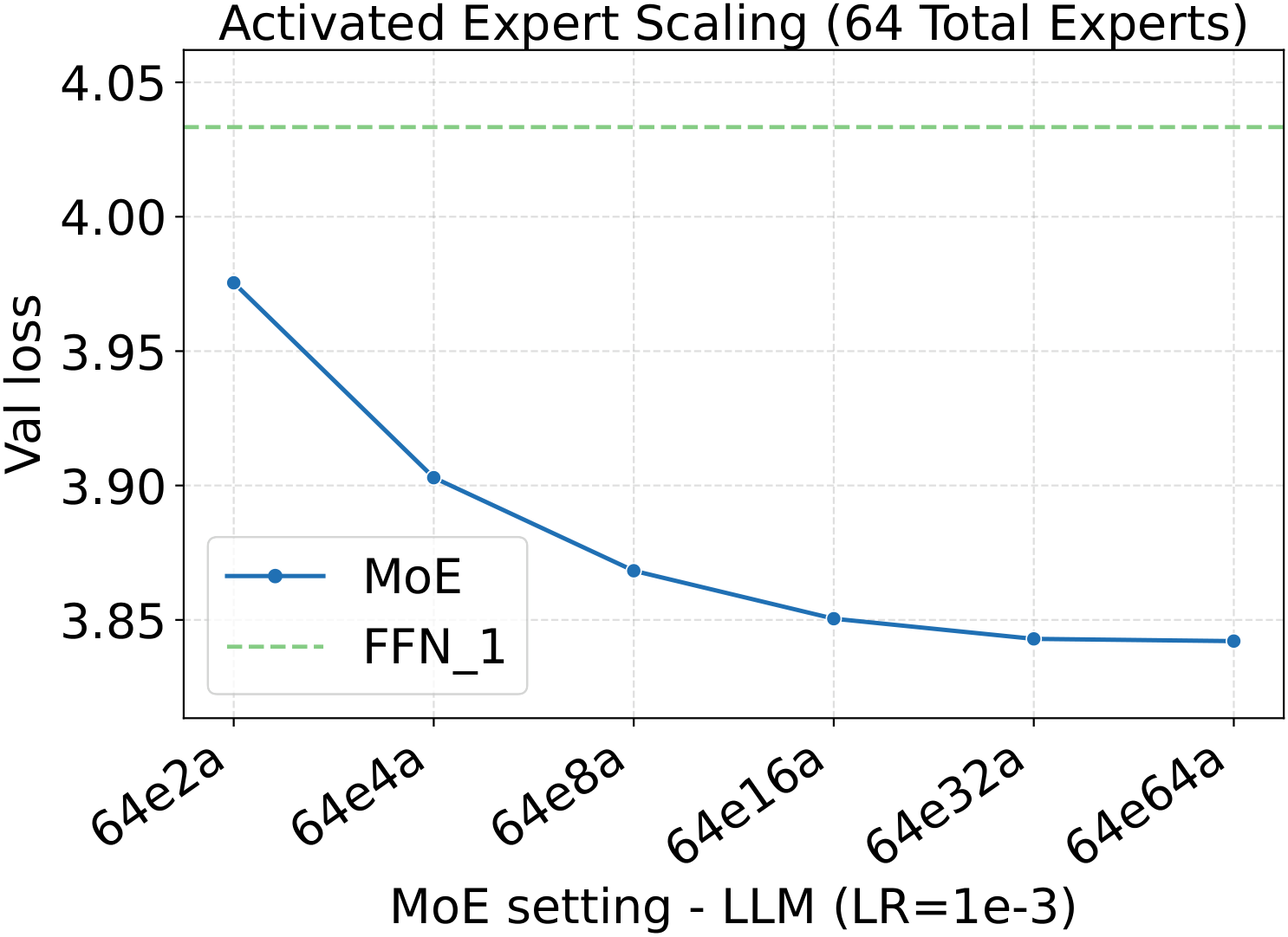
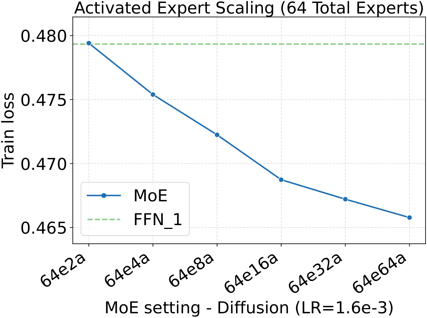
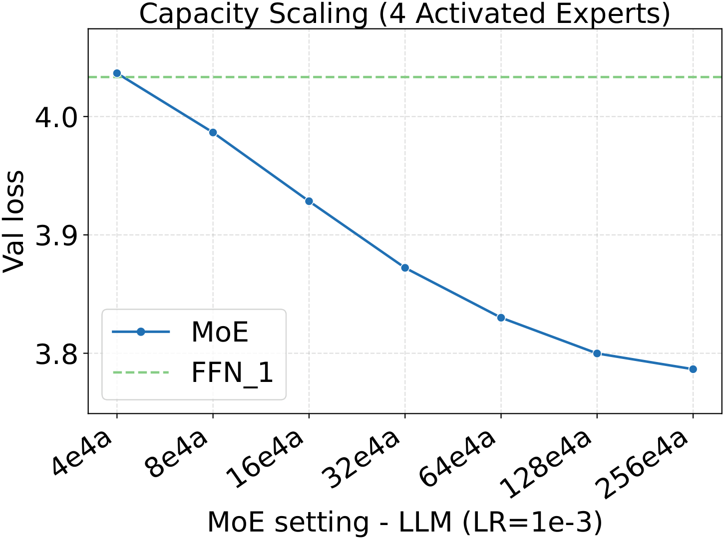
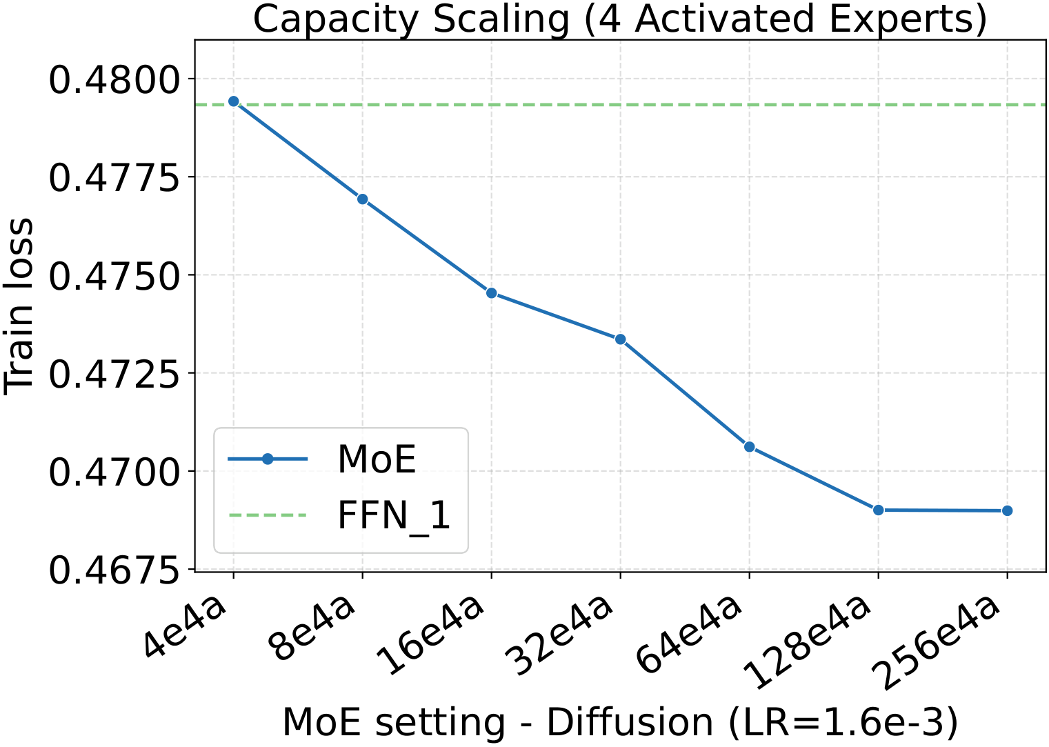
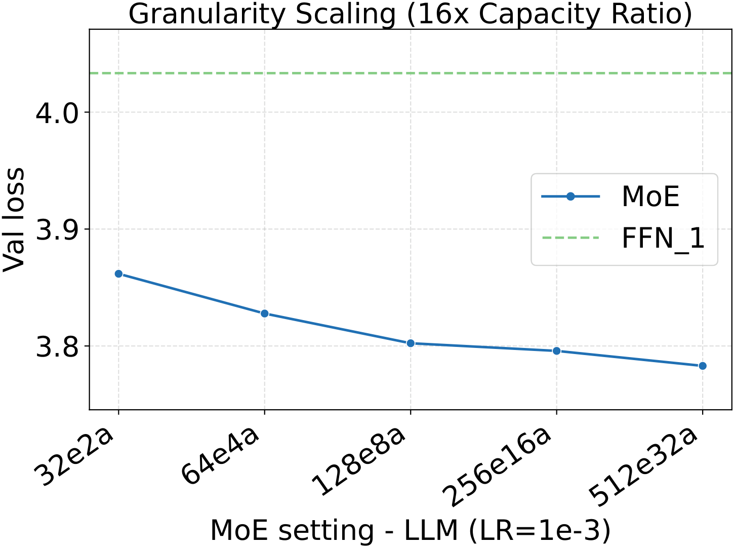
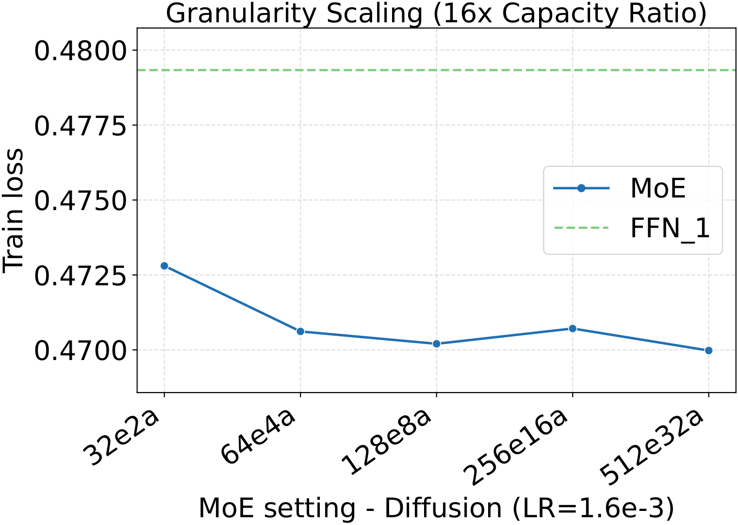
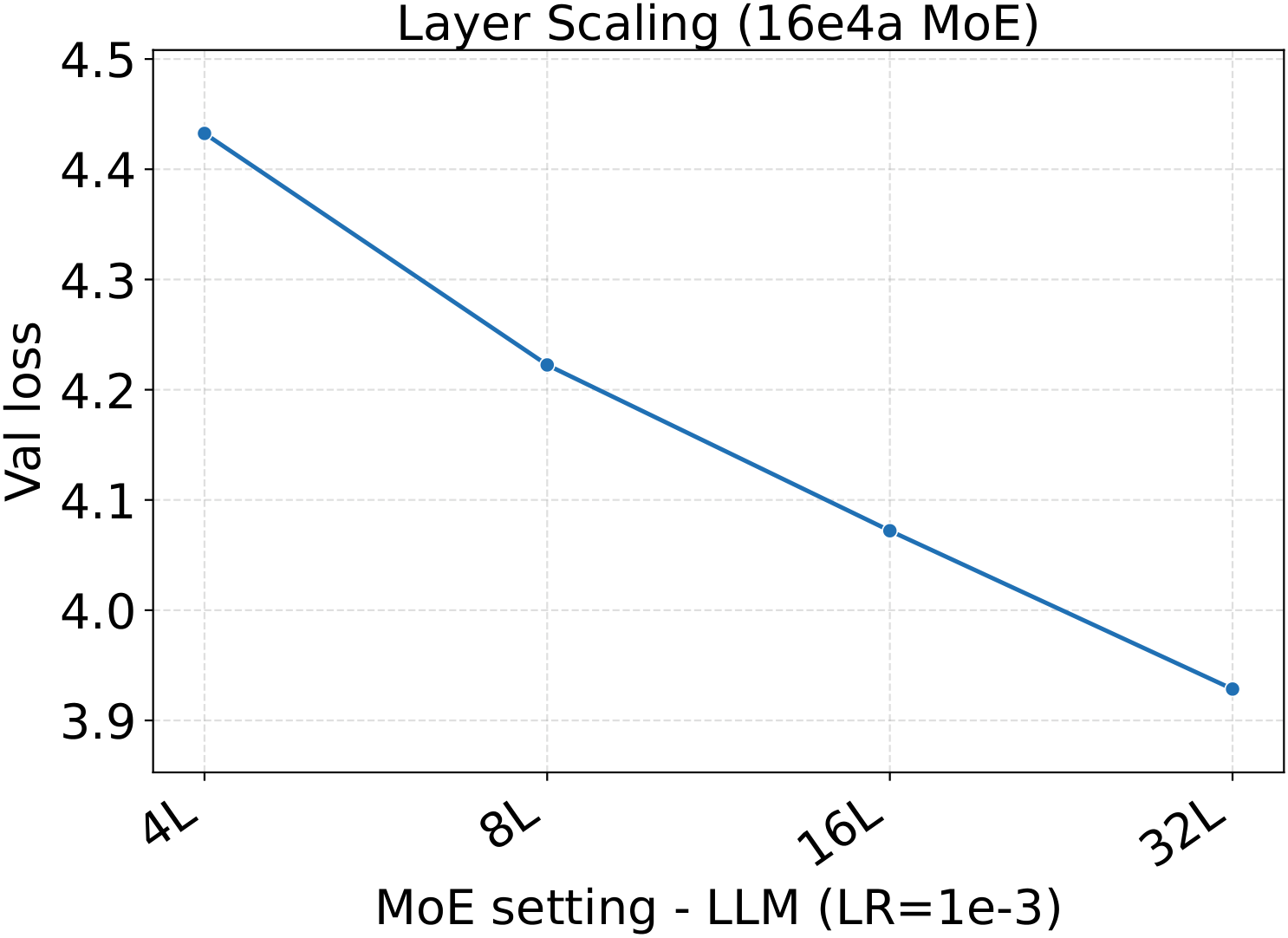
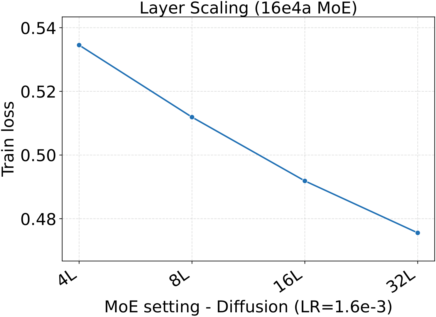
One pattern stands out across the four panels: capacity scaling (more total experts at fixed activated count) drives substantially lower loss than granularity scaling at the same fixed hyperparameters. Among the MoE quality knobs, total-expert count is the strongest lever per unit of training compute — which, conveniently, is also the cheapest one to scale, as we'll see in the systems benchmark below.
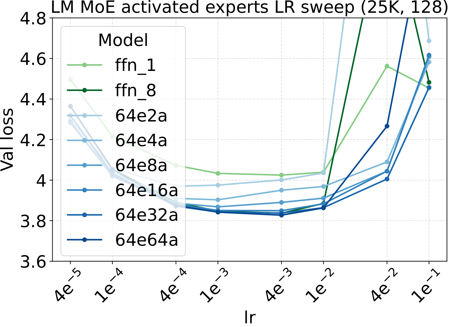
Activated experts: optima align across LR, WD, init, and the initial loss curve
The fixed-LR test above is the headline. The next two subsections answer the natural follow-up question: why is fixed-LR scaling so clean? Because the LR/WD/init optima are themselves stable across MoE configurations. Start with the most theory-loaded axis: the activated-expert count $a$ (Bridge II in the recipe). We sweep the three AdamW hyperparameters (LR, WD, init std) plus the initial-training-loss trajectory, all at fixed total experts and per-expert width:
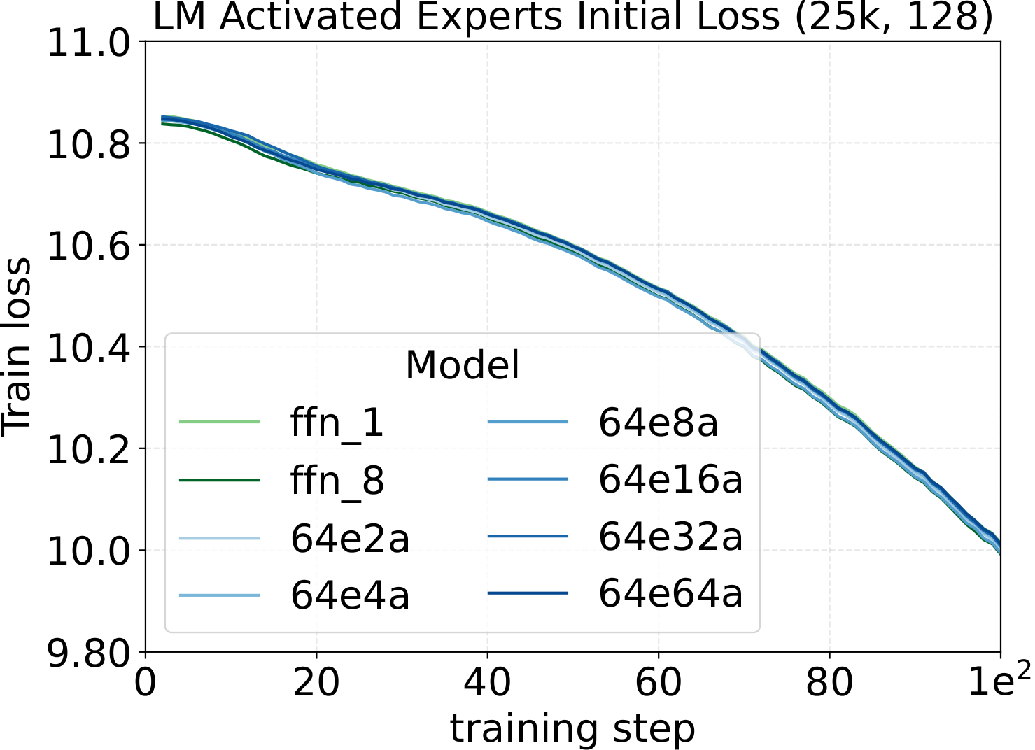
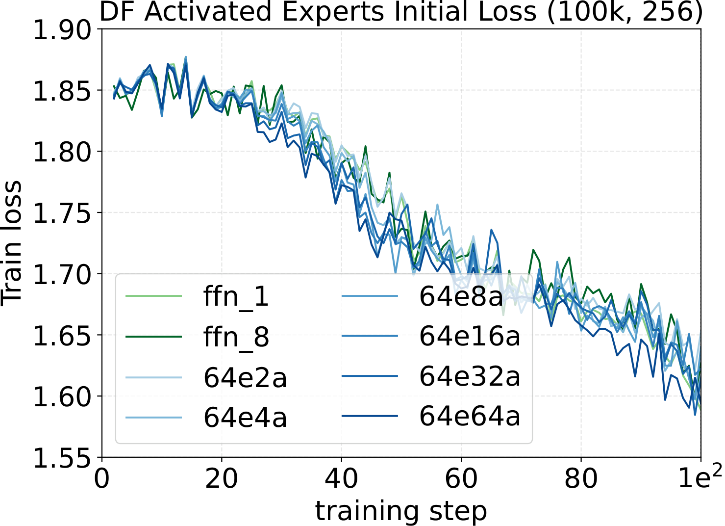
Practical implementation check. The initial training-loss curve (first ~100 steps) is the simplest tool to verify a $\mu\text{P}$ / Complete-muE implementation is correct. If the per-layer multipliers, output multiplier $A$, route scale $R$, and down-projection init are all wired up correctly, the initial-loss trajectories of dense and any MoE variant — across different activated counts, total experts, granularity, or backbone width — should stay close. They don't have to lie on top of each other; a small spread is expected from finite-batch noise and ordinary training stochasticity. What matters is the shape of the gap: the curves should track each other tightly with no widening trend. A persistent or growing separation in those first ~100 steps usually means one of the multipliers is off — wrong tensor axis, missing factor, or applied to the wrong projection. We use this as a quick unit test on every new MoE architecture: implement the variant, run ~100 steps at the dense-tuned hyperparameters, and overlay the curve on the dense baseline. If they track, the parameterization is fine; if they diverge clearly, find the bug before scaling up.
LR optima persist across the other MoE architectural axes
Bridge II covered activated experts. The follow-up question is whether the same LR transfer holds for the other MoE architectural knobs — capacity (total experts $N$), fixed-density granularity, shared experts, group-balanced routing, depth, and backbone width. We sweep each axis individually, with Complete-muE applied first and only the base LR scanned. The optima stay aligned across all six axes for both LM and diffusion:
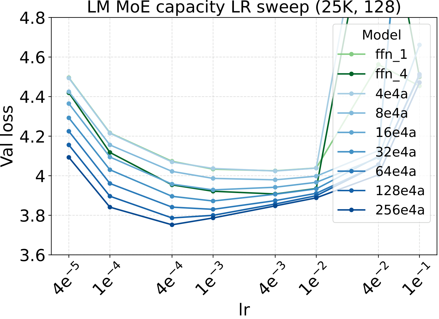
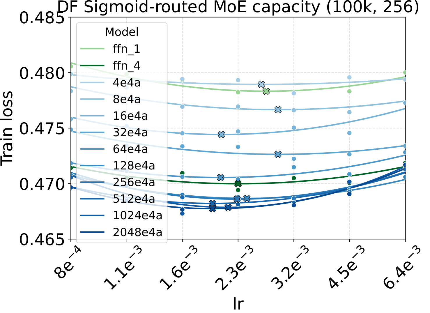
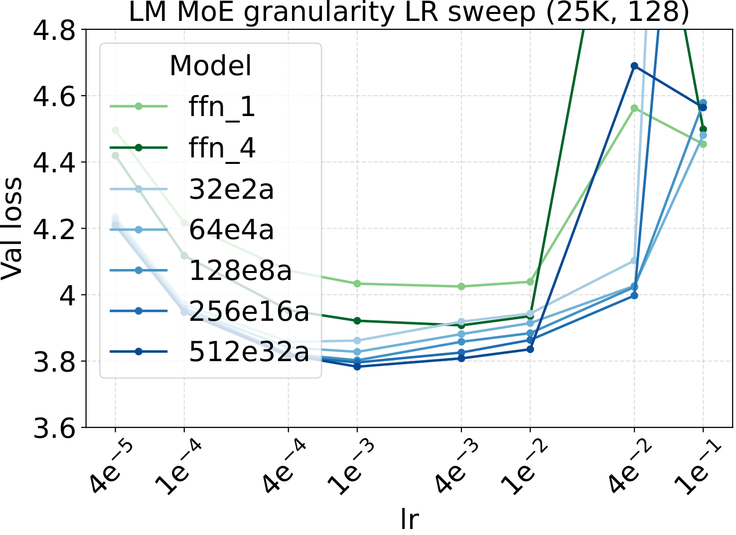
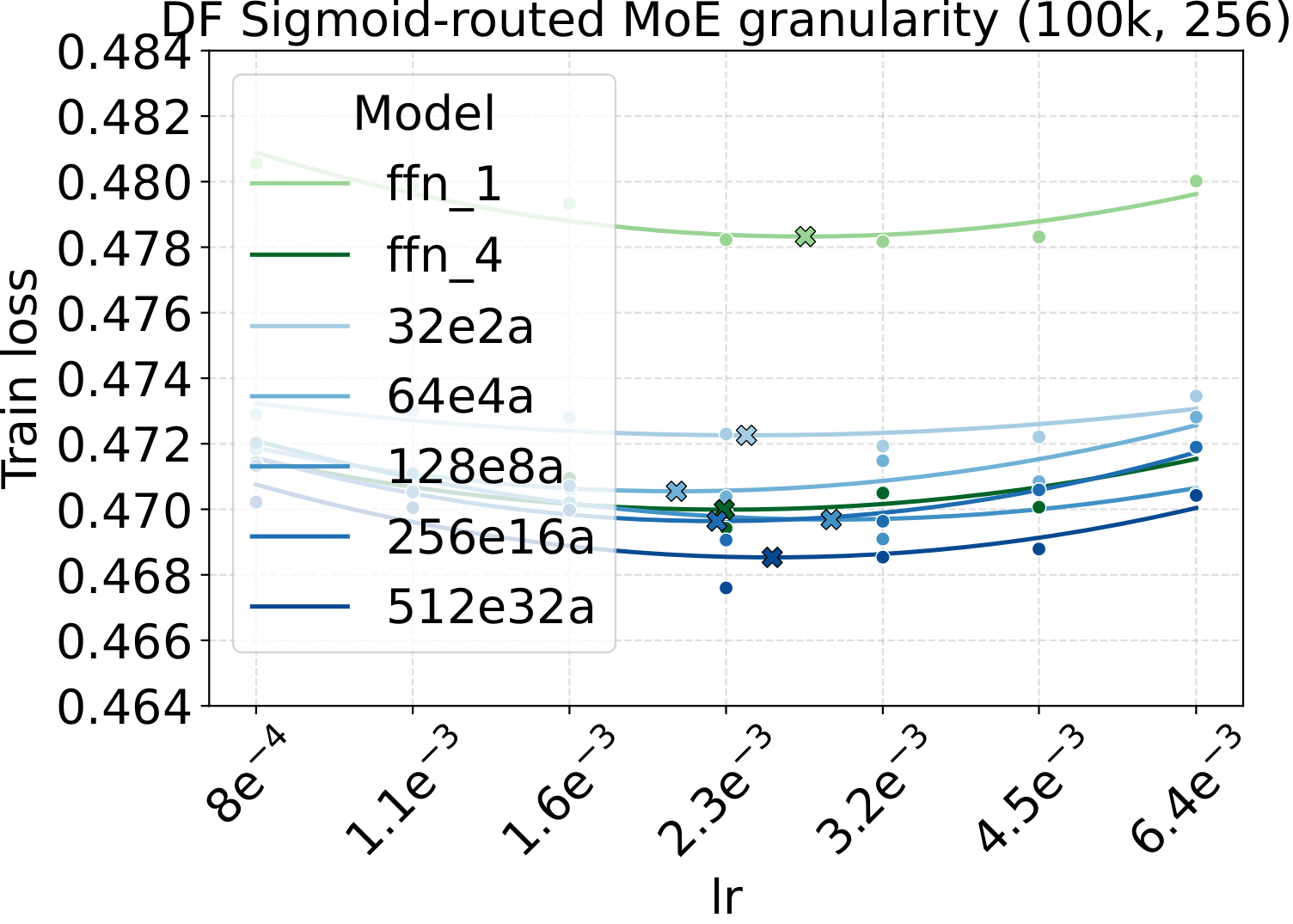
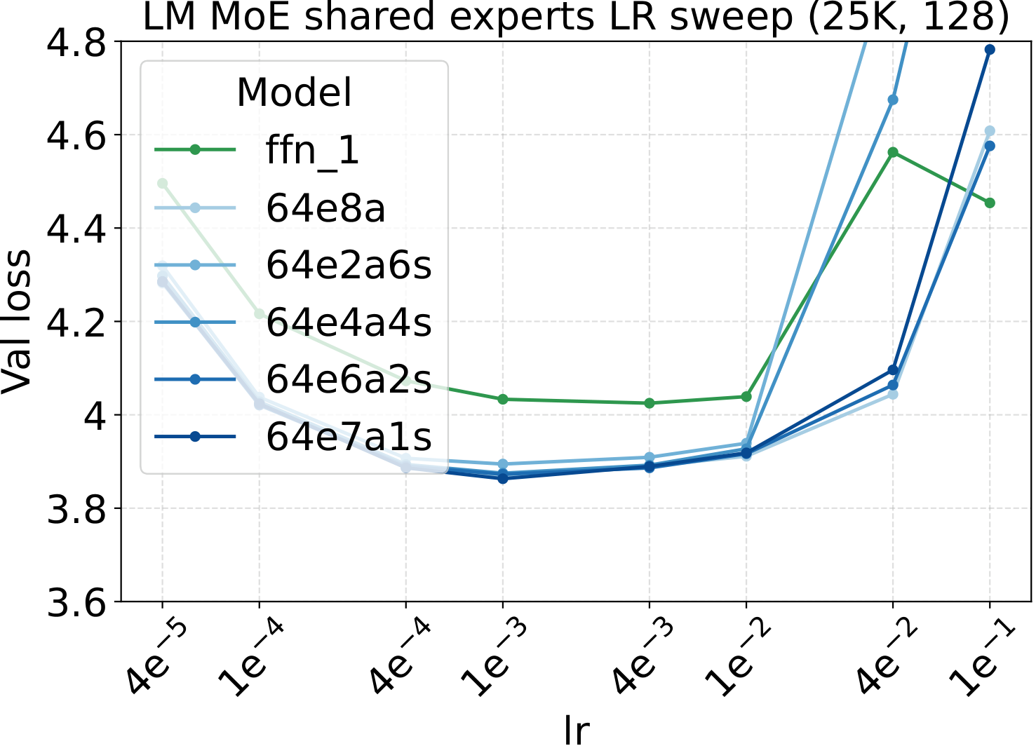
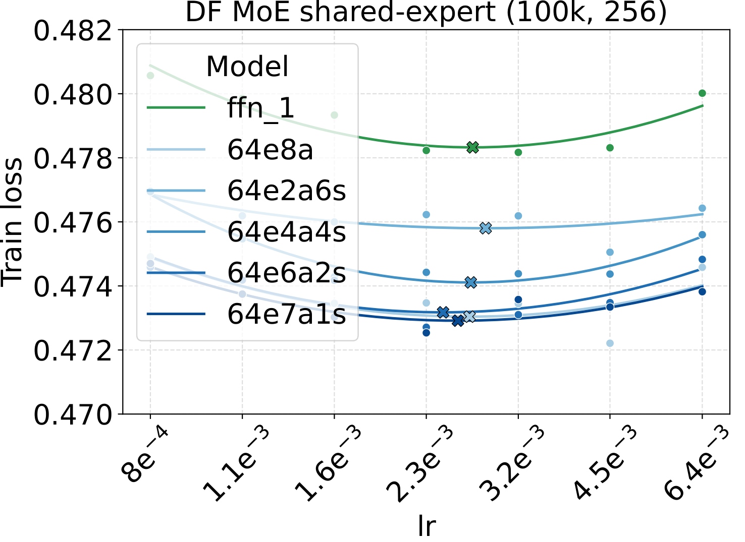
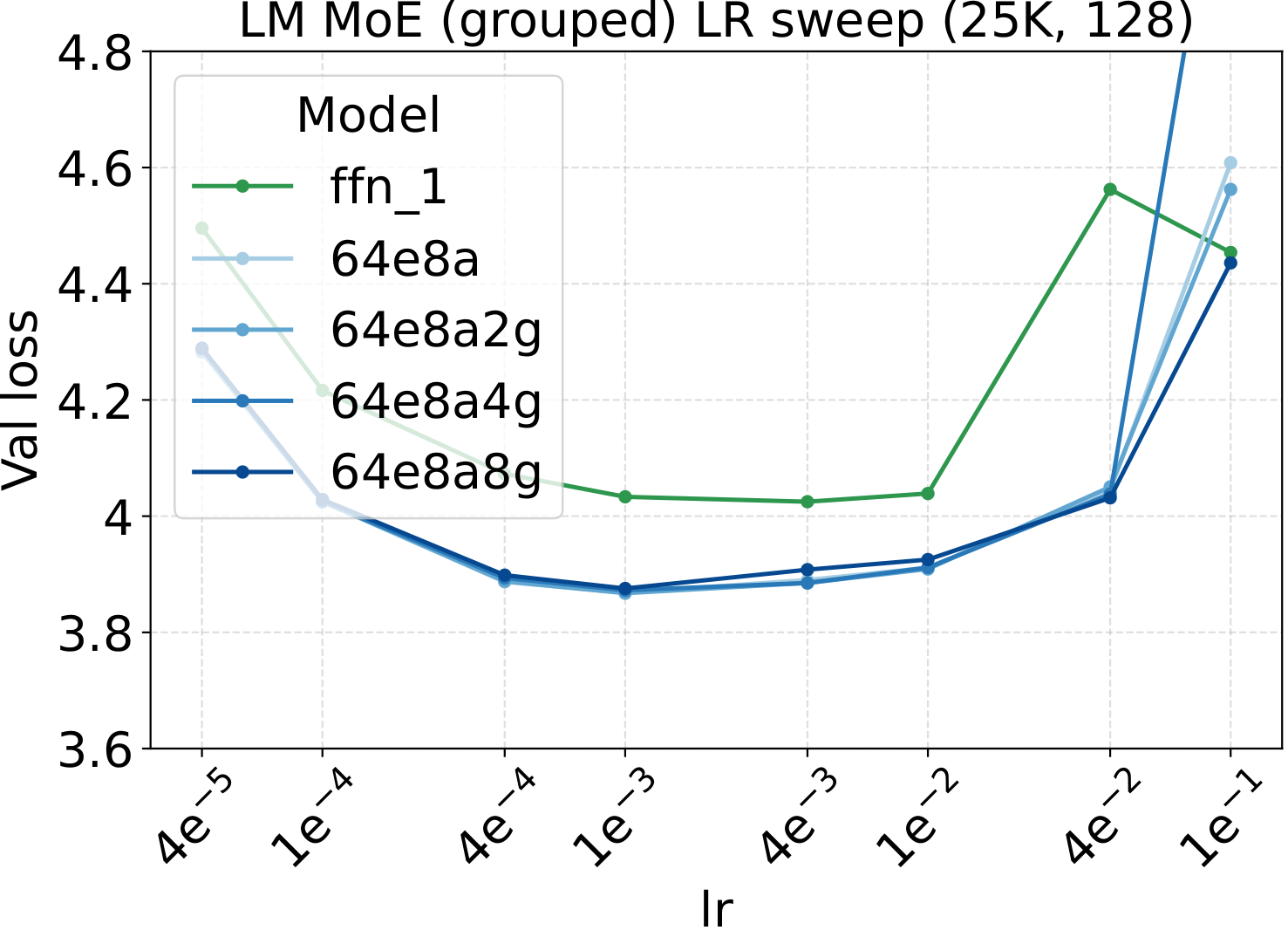
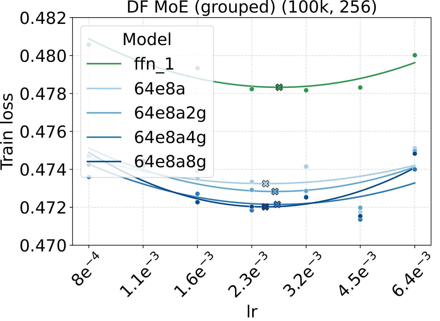
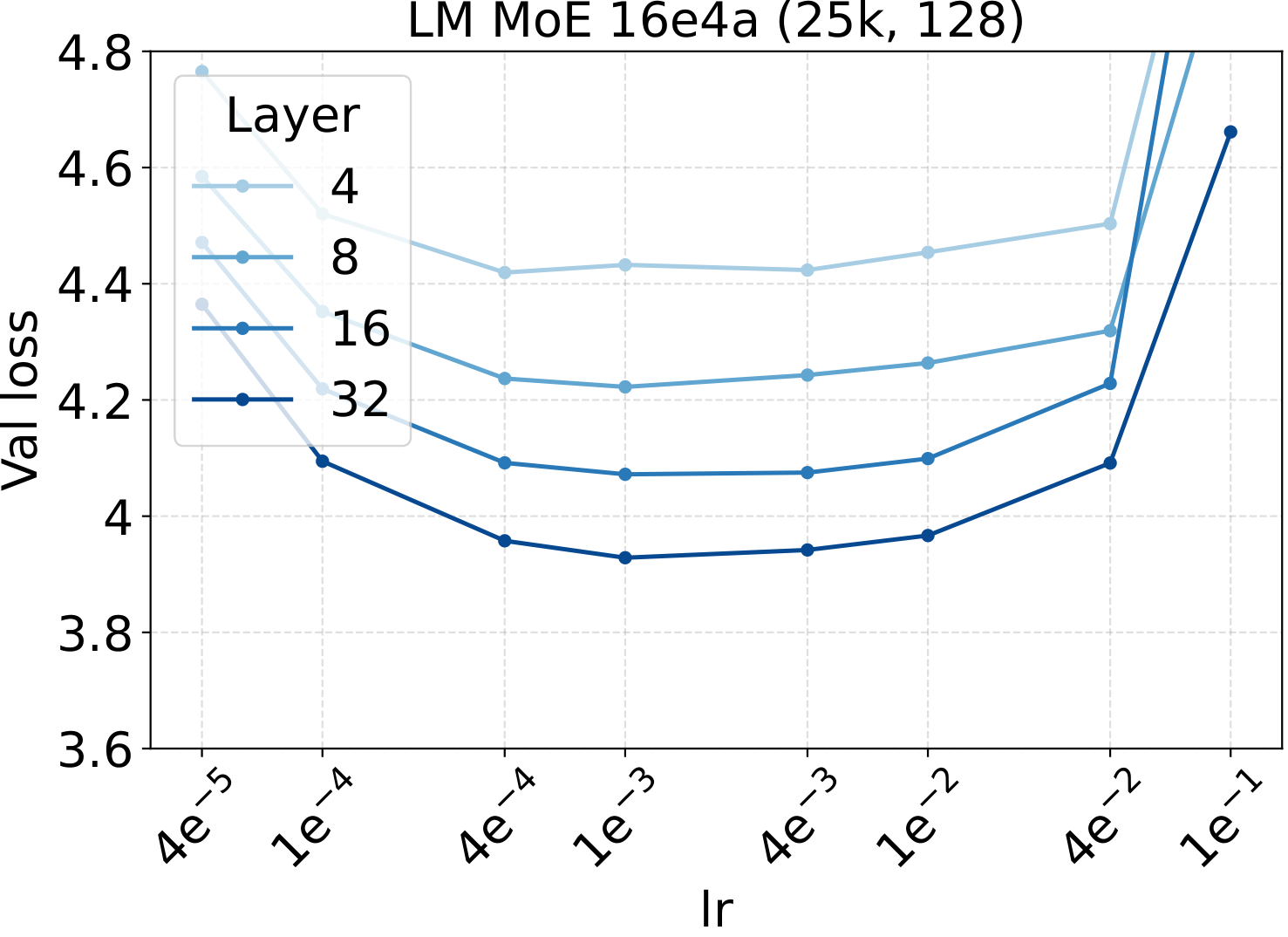
Combined with the activated-experts sweep above, this covers every MoE architectural axis the paper studies. The takeaway is uniform: once Complete-muE plugs the dense-tuned hyperparameters into the new architecture, the LR optimum stays put. There is no per-axis re-tuning step.
What's actually going on under the recipe
If you walked through the worked example, you already used both bridges: Step 2 (the MoE layer rule) is Bridge I — active-width $\mu\text{P}$ — and Step 1 (the global batch/duration rescaling) plus the implicit per-expert workload accounting is what Bridge II handles. The next two sections name the two operations, explain why each works at first order, and then flag the one second-order effect — a bounded $\sigma_0$ drift — that keeps the transfer honest rather than miraculous.
The core insight: active width + expert workload
Complete-muE's main observation is that you can take the messy MoE design space and decompose it into two clean, well-understood steps. Each step changes one thing.
Step 1 — Active width. A sparse MoE block that uses $a$ experts of width $h$ behaves, to first order, like a dense FFN with hidden width $H_a = a \cdot h$. This single quantity — the active width — governs everything that classical $\mu\text{P}$ knows how to handle.
Step 2 — Expert workload. Once active width is held fixed, the only remaining thing that changes when you flip between dense and sparse, or vary the activated-expert count, is how many tokens each expert sees per step. That's exactly the SDE setting — but applied to the per-expert training process rather than the whole model.
Decomposing the problem this way is the entire trick. Each step is a known problem with a known answer. The hard MoE-specific cases — total expert count, granularity, hybrids with shared experts and group-balanced routing — turn out to be compositions of these two steps. Nothing new needs to be invented for them.
Two bridges from dense to any MoE
The teaser figure at the top of this post is the picture of these two bridges: the two green diagonal arrows of the triangle are Bridge I (left, marked $\mu\text{P}$) and Bridge II (right, marked $\mu\text{P}$ + SDE); the red dashed bar at the bottom is the direct dense-to-sparse jump that doesn't transfer.
Bridge I: Dense FFN ↔ Dense MoE
The first bridge says: a dense FFN of width $H$ and a "Dense MoE" with $N$ experts of width $h = H/N$ (every expert active for every token) carry the same forward signal and the same per-step update size, as long as you do two small things:
- Use an output multiplier $A = d/H$ on the down-projection (where $d$ is the residual width). This is the standard $\mu\text{P}$ factor for a width-$H$ FFN.
- Use a route scale equal to the number of activated experts. Normalized routing averages expert outputs, which would otherwise shrink the update by $1/a$; the route scale undoes that.
Under the hood
For a unit-expansion dense companion at backbone width $d$, the matching rule for the FFN/MoE output branch is
$$A(H) = \frac{d}{H}, \qquad \sigma_{\mathrm{down}}(d, H) = \left(\frac{H}{d}\right)^{1/2} \sigma_{\mathrm{down}}^{(1)}(d), \qquad \eta_{\mathrm{down}}(d, H) = \eta_{\mathrm{down}}^{(1)}(d).$$
This is essentially $\mu\text{P}$ applied to the active width $H$, plus a normalized-route correction $r_a = a$.
Bridge II: Dense MoE ↔ Sparse MoE
The second bridge handles the move from a Dense MoE (all $N$ experts active) to a sparse MoE (only $a < N$ active). Once Bridge I is applied at the active width $H_a = ah$, the only remaining change is the per-expert data exposure.
Here's the elegant cancellation: when you switch from $a$ activated experts to $a'$ at fixed global batch size and steps, each expert's batch changes by the same factor as its training duration. Both go up or down together by $a'/a$. The standard SDE correction cancels:
Under the hood
$$\rho_B^{\mathrm{exp}} = \frac{B_{\mathrm{exp}}(a')}{B_{\mathrm{exp}}(a)} = \frac{a'}{a}, \qquad \rho_D^{\mathrm{exp}} = \frac{D_{\mathrm{exp}}(a')}{D_{\mathrm{exp}}(a)} = \frac{a'}{a}.$$
So the dense-style correction $\eta' \approx \eta\sqrt{\rho_B^{\mathrm{exp}}/\rho_D^{\mathrm{exp}}} = \eta$ — no first-order learning rate or weight decay multiplier is needed.
What does change is the expert-side noise-to-signal level $\sigma_0(a) = \eta \cdot \sigma_{\mathrm{exp}}(a)$, where $\sigma_{\mathrm{exp}}(a)$ is the per-expert gradient-noise standard deviation (which scales like $1/\sqrt{B_\mathrm{exp}(a)}$ with the per-expert batch). Making the MoE denser (larger $a$) lowers the per-step gradient noise, which is why denser MoEs can reach lower loss at the same hyperparameters — we return to this caveat in the next section.
Everything else is composition
That's it for new primitives. Every other MoE setting — total capacity, granularity, hybrid blocks with shared experts and grouped routing — is built by composing Bridge I and Bridge II:
- Total capacity ($N \to N'$): first widen the Dense-MoE companion (Bridge I), then re-sparsify back to $a$ active experts (Bridge II). The two factors cancel exactly.
- Granularity at fixed density ($s = a/N$): the active width is preserved by construction, so the same sparse-layer rule applies.
- Hybrid blocks (shared + grouped + routed): use one common active-width multiplier over the total active width $H_{\mathrm{tot}}$ and apply route scale only to routed branches.
Bridge II in practice: a second-order drift caveat
The first-order SDE correction in Bridge II cancels exactly, but there's a second-order effect we want to be upfront about: the per-step expert-side noise $\sigma_0(a)$ shifts when $a$ changes. The change is bounded:
$$\sigma_0(a') = \frac{\sigma_0(a)}{\sqrt{\rho_B^{\mathrm{exp}}}}.$$
This means Bridge II is not a strict SDE invariance — it's a relatively stable transfer with some mild residual drift in the optimal hyperparameters. The same kind of bounded drift shows up in two other places in the paper:
- Capacity scaling (varying $N$ at fixed $a, h$), because the composition that builds it uses Bridge II as a sub-step.
- Batch-size transfer at fixed training iterations, where the gradient noise $\sigma_0$ shifts even though the optimization horizon $H_{\mathrm{SDE}} = T\eta^2$ is preserved.
The empirical question is whether this drift is small enough to ignore in practice. The evidence in "Small-scale evidence" and "Large-scale evidence" — the activated-experts sweep, the architectural-axis sweeps, the fixed-LR scaling, and the large-scale runs at one shared hyperparameter setting — and the paper's calibration both answer yes.
Takeaways
- Small dense sweep, large MoE deployment. A single small-dense-proxy sweep is enough — no architecture-specific re-tuning at large scale.
- Two bridges, everything else by composition. Bridge I (active-width $\mu\text{P}$) + Bridge II (per-expert workload) cover the whole MoE design space without new primitives.
- The math is honest about its limits. The SDE cancellation is first-order, with a bounded second-order $\sigma_0$ drift. Small-scale sweeps and large-scale runs both confirm this drift is small enough in practice.
- Practical wins are real and measurable. $4.5\times$ on $240$P $5$s video and $5.3\text{-}5.5\times$ on LLM, all at the dense baseline's hyperparameters.
Why this matters
For teams training large MoE models, the cost of "what learning rate should I use for this new MoE configuration?" has historically been a hyperparameter sweep at scale. Complete-muE replaces that sweep with one table lookup. The savings compound every time a team tries a new sparsity, granularity, or hybrid routing variant.
For researchers, the contribution is conceptual: capacity, granularity, and hybrid routing aren't new primitive hyperparameter-transfer rules — they're compositions of two well-understood bridge cases. That decomposition is the part most likely to outlive any specific architecture trend.
The paper
Complete-muE: Optimal Hyperparameter Transfer and Scaling for MoE Models — Hongwu Peng, Ohiremen Dibua, Yuanjun Xiong, Yifan Gong, Jianming Zhang, Yan Kang (Adobe Research). Read the preprint on arXiv: arXiv:2605.23893.
Citation
Please cite this work as:
Peng, Hongwu and Dibua, Ohiremen and Xiong, Yuanjun and Gong, Yifan and Zhang, Jianming and Kang, Yan, "Complete-muE: Optimal Hyperparameter Transfer and Scaling for MoE Models", arXiv preprint arXiv:2605.23893, 2026.Or use the BibTeX citation:
@article{peng2026completemue,
  title={Complete-muE: Optimal Hyperparameter Transfer and Scaling for MoE Models},
  author={Peng, Hongwu and Dibua, Ohiremen and Xiong, Yuanjun and Gong, Yifan and Zhang, Jianming and Kang, Yan},
  journal={arXiv preprint arXiv:2605.23893},
  year={2026}
}
Questions? Email hongwup@adobe.com.
References
Foundational works Complete-muE builds on: $\mu\text{P}$-style transfer, SDE-based optimizer scaling, MoE-specific transfer, and the broader sparse-MoE literature. Citations marked in the body link to the corresponding margin note; the full list is here.
- Yang, G., Hu, E. J., Babuschkin, I., Sidor, S., Liu, X., Farhi, D., Ryder, N., Pachocki, J., Chen, W., & Gao, J. (2022). Tensor Programs V: Tuning large neural networks via zero-shot hyperparameter transfer. NeurIPS. arXiv:2203.03466.
- Dey, N. S., Zhang, B. C., Noci, L., Li, M., Bordelon, B., Bergsma, S., Pehlevan, C., Hanin, B., & Hestness, J. (2025). Don't be lazy: CompleteP enables compute-efficient deep transformers. NeurIPS. arXiv:2505.01618.
- Mlodozeniec, B., Ablin, P., Béthune, L., Busbridge, D., Klein, M., Ramapuram, J., & Cuturi, M. (2025). Completed Hyperparameter Transfer across Modules, Width, Depth, Batch and Duration. arXiv:2512.22382.
- Malladi, S., Lyu, K., Panigrahi, A., & Arora, S. (2022). On the SDEs and scaling rules for adaptive gradient algorithms. NeurIPS. arXiv:2205.10287.
- Małaśnicki, J., Ciebiera, K., Boruń, M., Pióro, M., Ludziejewski, J., Stefaniak, M., Krutul, M., Jaszczur, S., Cygan, M., Adamczewski, K., et al. (2025). Mu-Parametrization for Mixture of Experts. ES-FoMo III Workshop. arXiv:2506.16962.
- Jiang, T., Bordelon, B., Pehlevan, C., & Hanin, B. (2026). Hyperparameter Transfer with Mixture-of-Expert Layers. arXiv preprint.
- Shazeer, N., Mirhoseini, A., Maziarz, K., Davis, A., Le, Q., Hinton, G., & Dean, J. (2017). Outrageously Large Neural Networks: The Sparsely-Gated Mixture-of-Experts Layer. ICLR. arXiv:1701.06538.
- Fedus, W., Zoph, B., & Shazeer, N. (2022). Switch Transformers: Scaling to Trillion Parameter Models with Simple and Efficient Sparsity. JMLR. arXiv:2101.03961.
- Dai, D., Deng, C., Zhao, C., Xu, R. X., Gao, H., Chen, D., Li, J., Zeng, W., Yu, X., Wu, Y., et al. (2024). DeepSeekMoE: Towards Ultimate Expert Specialization in Mixture-of-Experts Language Models. ACL. arXiv:2401.06066.
- Zheng, C., Lou, A., Liu, C., Wei, X., Liu, Z., & Ermon, S. (2025). Scaling Diffusion Transformers Efficiently via $\mu\text{P}$. NeurIPS. arXiv:2505.15270.
- DeepSeek-AI. (2024). DeepSeek-V3 Technical Report. arXiv:2412.19437.
- Orvieto, A., De, S., Gulcehre, C., Pascanu, R., & Smith, S. L. (2025). In Search of Adam's Secret Sauce. NeurIPS. arXiv:2510.08198.